A near-zero return-count diagnostic for fund valuation patterns, with explicit zero, sample-volatility and denominator conventions.
Bias ratio
The bias ratio is a return-distribution diagnostic that compares the number of small nonnegative returns with the number of small negative returns. It helps a fund analyst notice an unusually lopsided pattern near zero that deserves investigation into valuation and liquidity. Adil Abdulali developed the measure; Riskdata subsequently incorporated it into its hedge-fund risk analysis. A high value is a diligence signal, not proof of fraud. Riskdata’s original explanation explicitly separates return smoothing from unfair manipulation.
The “bias” concerns the shape of reported returns, rather than bias in a regression coefficient.
A fund’s net asset value can depend on estimates when its holdings rarely trade. If valuation discretion repeatedly keeps reported returns just above zero, the nearby positive count may become unusually large relative to the negative count. The useful question is then what produced the imbalance?
State the counting rule first
For monthly simple returns r1,…,rn, let s be their standard deviation. One explicit count-based convention is
Here K>0 is an added denominator count that prevents division by zero. The bins are anchored at zero, not at the sample mean; s controls their width. Returns exactly at −s and +s are included, while zero belongs only to N+.
This follows the interval prose in Abdulali’s published patent application, detailed description. That source’s displayed denominator inconsistently shows a closed interval including zero. Consequently, endpoint rules must be reported rather than assumed to be universal. It also specifies a positive K without fixing it to one. This article chooses K=1 and the sample standard deviation with divisor n−1; these are declared calculation choices, not a claim that every implementation agrees.
Eight months, three possible answers
Consider these fictional monthly returns, in percent:
Month
1
2
3
4
5
6
7
8
Return
−2.0
−1.0
−0.5
0.0
0.1
0.2
0.3
3.0
The sample standard deviation is s≈1.4337%. Count all eight months when calculating s, including the two observations outside the eventual counting bins.
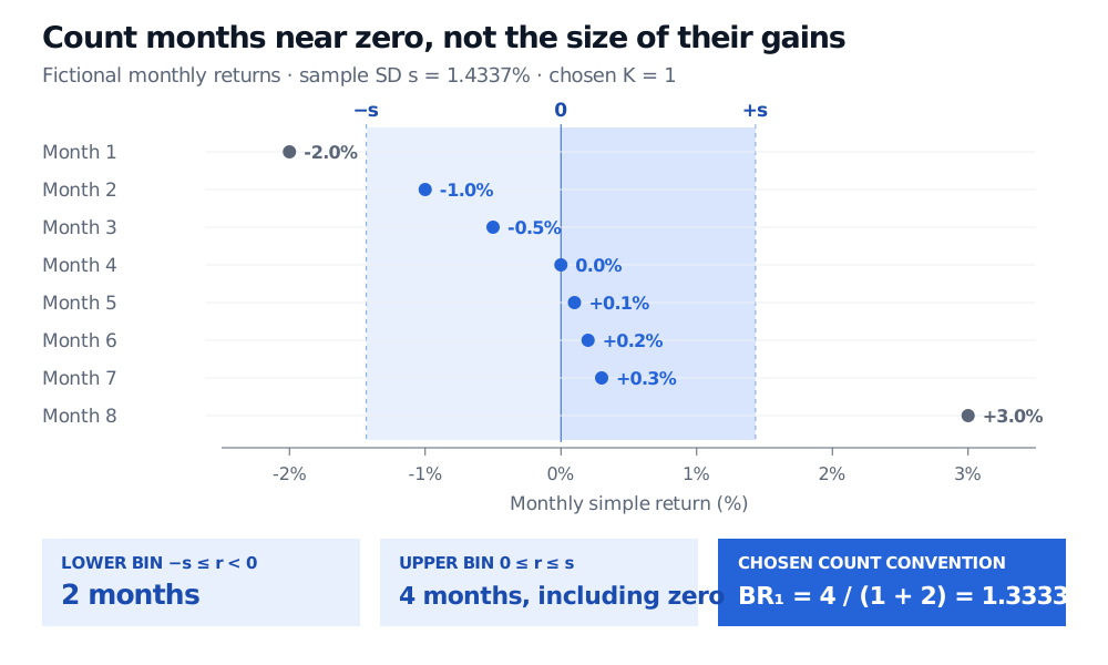
The upper bin contains 0.0%,0.1%,0.2%,0.3%: four months.
The lower bin contains −1.0%,−0.5%: two months.
The −2.0% and 3.0% months affect the estimated width but neither count.
Thus the chosen statistic is
BR1=1+24=34≈1.3333.
Eight fictional monthly returns plotted against zero and plus or minus sample SD 1.4337 percent; four months enter the upper bin and two enter the lower bin, giving BR1 of 4 divided by 3.
Fictional monthly returns: the zero month enters the upper bin only; the added denominator count changes the ratio from 2 to 1.3333.
The raw quotient without an added count would be 4/2=2. Keeping K=1 but including zero in the lower bin as well would give 4/(1+3)=1. These are different calculations on identical observations. A reported “bias ratio” without its zero rule and denominator convention is incomplete.
The added count matters particularly in short samples. If N−=0, this convention returns N+/K, whereas the raw quotient has a zero denominator. A finite answer does not create evidence that a sparse sample lacks. With fewer than two observations the sample SD is unavailable; with s=0 the bins collapse, so the diagnostic should not receive the usual near-zero-distribution interpretation.
Read the pattern in its economic context
Riskdata’s strategy comparison stresses comparison with funds trading similar assets and facing similar liquidity. An imbalance can reflect genuine positive carry or the economics of the strategy as well as subjective marks. Comparing a liquid equity strategy with an illiquid credit strategy against one universal cutoff discards that context. The ratio supplies neither a fraud probability nor a calibrated pass/fail test.
Precision also matters: rounding a small negative observation to zero moves it from the lower count to the upper count under our rule. Sample length, reporting frequency, fees and valuation policy therefore belong beside any comparison. A few monthly counts should not be read as a stable population characteristic.
This statistic ignores time order: rearranging the same returns leaves both s and the counts unchanged. Autocorrelation asks a separate question about how returns follow one another. For that complementary perspective, see Serial Correlation: Durbin–Watson, Breusch–Godfrey, and Newey–West (public preview; full lesson requires membership). Its regression diagnostics do not turn the bias ratio into a formal manipulation test.