Benign overfitting: Definition & Examples

Benign overfitting is the phenomenon in which a predictor fits noisy training observations exactly yet predicts nearly as well as the underlying signal rule. In an asymptotic formulation, its excess prediction risk tends to zero as sample size grows. For a quant researcher, zero training error therefore leaves a question unanswered: what happens on fresh data? Bartlett and colleagues characterise this possibility for minimum-norm linear regression.

“Benign” refers to excess risk

Take the correctly specified model $y=x^{\top}\beta^{*}+\varepsilon$ , with $\mathbb{E}[\varepsilon\mid x]=0$ , constant conditional noise variance $\sigma^{2}>0$ , and finite second moments. For a fitted coefficient vector $\hat\beta$ , evaluated on a fresh observation independent of training, expand the square:

\begin{aligned} \mathbb{E}[(y-x^{\top}\hat\beta)^2\mid\hat\beta] &=\sigma^{2}+\mathcal{E}(\hat\beta),\\ \mathcal{E}(\hat\beta) &=(\hat\beta-\beta^{*})^{\top}\Sigma(\hat\beta-\beta^{*}), \qquad \Sigma=\mathbb{E}[xx^{\top}]. \end{aligned}

The cross-term vanishes by the conditional mean-zero assumption. With centred features, $\Sigma$ is the covariance matrix. Benign overfitting asks for $\mathcal{E}(\hat\beta)\to0$ , not total test MSE tending to zero: irreducible noise remains. Nor does small prediction risk require every coefficient error to be small; the covariance weights errors by how much those directions vary on new observations.

The bias–variance derivation develops the fresh-noise distinction in detail (full lesson requires membership; public preview available).

A perfect fit that fails

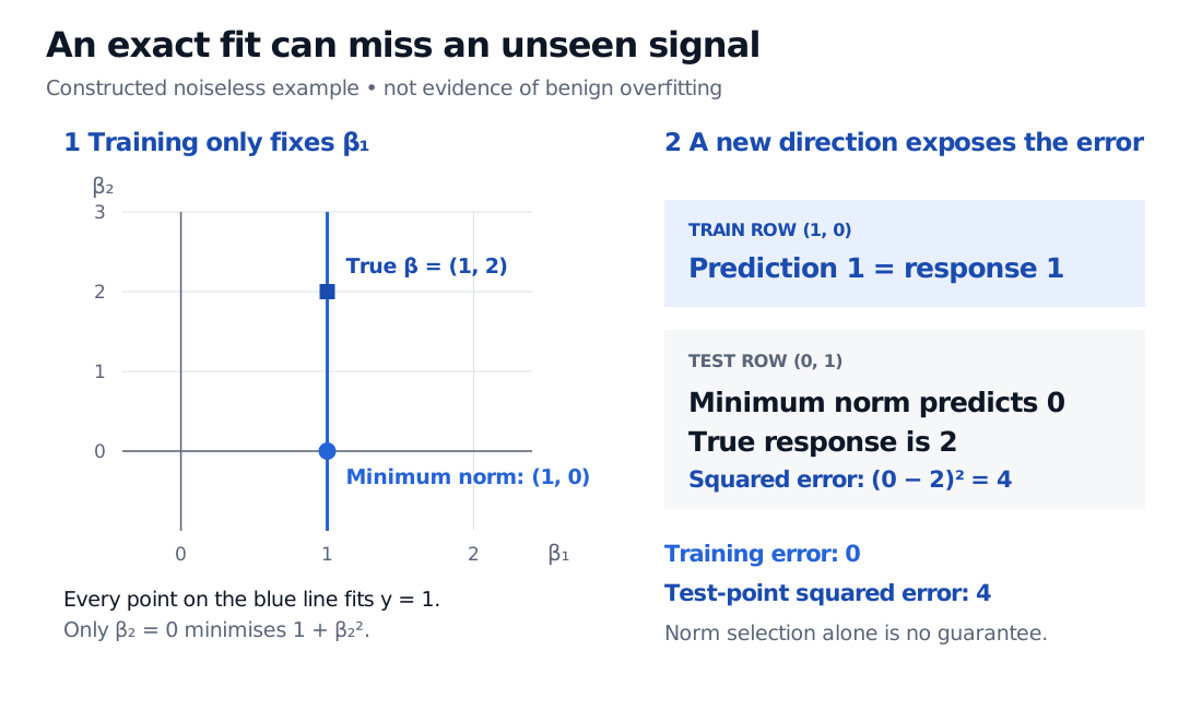
Here is a deliberately finite, noiseless counterexample to the claim that interpolation plus minimum norm guarantees good prediction. Use one training row $X=(1,0)$ and response $y=1$ . Every vector

\beta=(1,t),\qquad t\in\mathbb{R},

fits exactly because $X\beta=1$ . Minimising the squared Euclidean coefficient norm $1+t^{2}$ picks $\hat\beta=(1,0)$ .

Suppose the true coefficient vector is $\beta^{*}=(1,2)$ . It agrees with the training observation. At the test row $x_{\mathrm{test}}=(0,1)$ , however,

\hat y=0,\qquad y^{*}=2,\qquad (\hat y-y^{*})^{2}=4.

Constructed noiseless counterexample: training row (1, 0) with response 1 permits every coefficient vector (1, t). Minimum Euclidean norm chooses (1, 0), while the true vector is (1, 2). At test row (0, 1), prediction 0 misses truth 2 and gives squared error 4.

An original counterexample, not a benign-overfitting experiment. The blue line contains all exact training fits; minimum norm chooses a point that misses the unobserved signal direction.

The sample contains no information about the second coefficient. A norm preference resolves the ambiguity, but it cannot establish that zero is the true value. “Minimum norm” also refers to a specified feature representation and scaling; changing them changes the selection rule. This single test-point error is not a population-risk estimate or an asymptotic result.

What can make interpolation harmless?

In the paper’s linear setting, a sufficiently broad tail of small covariance eigenvalues can distribute fitted label noise across directions that contribute little to prediction risk. Signal distortion must also vanish: the noise-fitting condition alone is insufficient. The theorem uses independent training observations, distributional tail assumptions and rank conditions—not parameter count alone.

One concrete sufficient construction follows from its Theorem 4. For each $n$ , use $p_n=n^{2}+1$ centred Gaussian features with covariance eigenvalues

1,\quad \underbrace{n^{-3/2},\ldots,n^{-3/2}}_{n^{2}\text{ entries}}.

Assume i.i.d. training pairs, independent Gaussian label noise with fixed positive variance, and true coefficient vectors whose Euclidean norms stay bounded. This is a sequence of changing feature spaces and covariances, not repeated fitting of one fixed dataset.

To check the construction, define the paper’s tail ranks for decreasing eigenvalues $\lambda_j$ :

r_k=\frac{\sum_{j>k}\lambda_j}{\lambda_{k+1}},\qquad R_k=\frac{(\sum_{j>k}\lambda_j)^2}{\sum_{j>k}\lambda_j^2}.

Direct summation gives

r_0=1+\sqrt n

and

r_1=R_1=n^{2}

. For the theorem’s fixed constant

b>1

, the first index with

r_k\ge bn

k^{*}=1

eventually, not necessarily at a particular finite sample size. Thus

\frac{r_0}{n}=\frac{1+\sqrt n}{n}\to0,\qquad \frac{k^{*}}{n}=\frac1n\to0,\qquad \frac{n}{R_{k^{*}}}=\frac1n\to0.

Under these assumptions, the theorem yields vanishing excess risk in probability. Here $R_1$ describes the small-eigenvalue tail; it is not $R_0$ , which grows only on the order of $n$ . Neither the construction nor the counterexample proves success at a chosen finite $n$ .

Reading a financial modelling result

A low-variance feature direction is not automatically irrelevant: its coefficient and alignment with the signal matter, as the counterexample shows. Financial observations can also be dependent, and their feature covariance can change over time. Those features of a research problem need separate treatment before applying an i.i.d. theorem.

Out-of-sample evaluation still has to assess the fitted rule and the selection process. A double-descent curve describes how error changes across model sizes or training stages; benign overfitting describes the quality of interpolating prediction. Observing a second descent does not by itself establish vanishing excess risk.

Sources

Bartlett, P. L., Long, P. M., Lugosi, G. and Tsigler, A. (2020), Benign Overfitting in Linear Regression. Definitions 1–3 specify the model, estimator and effective ranks; Theorem 4 and §3.1 supply the sufficient-risk conditions used above. Published in PNAS, 117(48), 30063–30070.

“Benign” refers to excess risk

A perfect fit that fails

What can make interpolation harmless?

Reading a financial modelling result

Sources

Related terms

Double descent