Sequential search using a probabilistic surrogate and acquisition rule: expected improvement, uncertain incumbents and time-aware assessment of the entire search.
Bayesian optimisation
Bayesian optimisation is a sequential method for choosing where to evaluate an expensive objective by using a probabilistic model of that objective and an acquisition rule. In quant research, it can allocate a limited training or simulation budget to promising hyperparameter configurations. Saving evaluations does not make the selected backtest an unbiased estimate of future performance.
A model of the search, separate from the trading model
Suppose x contains a model's settings and f(x) is its validation score under a fixed evaluation protocol. Evaluating f may require fitting the whole forecasting pipeline across several historical windows. Bayesian optimisation builds a cheaper surrogate for this mapping from settings to scores. A Gaussian process is one common surrogate; the method is broader than that particular model.
The loop is to evaluate an initial set of configurations, update the surrogate, choose the next configuration by maximising an acquisition function, evaluate the real objective there, and repeat within the budget. The acquisition function assigns value to an evaluation using the surrogate's predictions and uncertainty. It can therefore favour a region with an uncertain score over the region with the highest predicted score. Snoek, Larochelle and Adams develop this approach for machine-learning experiments.
The surrogate models f(x); it is not itself necessarily the forecasting model being tuned. Its posterior distribution describes uncertainty about the objective conditional on the evaluations and modelling assumptions. The GP regression lesson derives predictive means and variances; its full teaching requires membership, with a public preview available.
Expected improvement: a value for the next evaluation
Consider maximisation, noiseless evaluations and a known incumbent f∗ equal to the best objective value observed so far. Suppose the surrogate marginal at a candidate is
f(x)∣D∼N(μ(x),σ2(x)),
where D contains previous evaluations and σ is a posterior standard deviation. Improvement is the positive part of beating the incumbent:
I(x)=max{f(x)−f∗,0},EI(x)=E[I(x)∣D].
With zero exploration offset and σ(x)>0, the normal expectation gives
EI(x)=(μ(x)−f∗)Φ(z)+σ(x)ϕ(z),z=σ(x)μ(x)−f∗,
where Φ and ϕ are the standard normal CDF and density. When σ(x)=0, use max{μ(x)−f∗,0} directly; dividing by zero is unnecessary. Jones, Schonlau and Welch's EGO paper, §4.1, presents EI for minimisation. The signs above reverse that convention. EI measures expected improvement in objective units, rather than only the probability of beating f∗.
Take three candidate configurations and an incumbent of 0.025. All scores below are dimensionless. These are stipulated surrogate posteriors, not values obtained by fitting a GP or measuring strategy returns.
Candidate
Posterior mean
Posterior SD
Expected improvement
A
0.030
0.010
0.006977965574
B
0.020
0.030
0.009634110646
C
0.010
0
0
For A, z=(0.030−0.025)/0.010=0.5. For B, z=(0.020−0.025)/0.030=−1/6. Substitution produces the table. C is certain under the stipulated surrogate and below the incumbent, so its EI is zero.
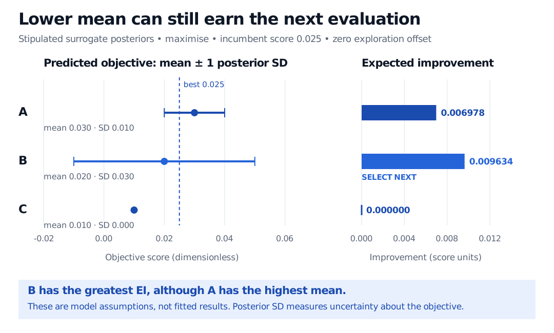
B receives the next evaluation, even though A has the higher posterior mean. B's greater uncertainty leaves enough probability mass above the incumbent to give the larger expected improvement. This is a model-based reason to investigate B, not evidence that B's unknown objective actually exceeds A's. It is also not a final recommendation to deploy B.
Stipulated dimensionless objective to maximise: A has mean 0.030, posterior SD 0.010 and EI 0.006978; B has mean 0.020, SD 0.030 and EI 0.009634 and is selected next; C has mean 0.010, SD zero and EI zero. The incumbent is 0.025. Left segments show mean plus or minus one posterior SD.
Original stipulated example. Posterior uncertainty about the objective determines EI; the intervals are not return-volatility estimates or guarantees about the unknown score.
Here σ measures epistemic uncertainty about the objective under the surrogate. It is not the volatility of a strategy's realised returns. An uncertain score can justify collecting information while the corresponding strategy remains unsuitable for trading.
Conventions change the acquisition
Real validation scores can vary with training randomness, sampled folds or simulation error. With noisy evaluations, the largest observed score need not be the best underlying objective. A plug-in rule using the best posterior mean and a noisy-EI rule integrating uncertainty about previously evaluated values are different constructions. Letham and colleagues, §§2.1 and 3.2, explain the distinction. The simple table uses neither variant: its incumbent is treated as known.
Declare the direction, score scale, noise model, incumbent rule and any exploration offset. Respect feasible settings and resource constraints. Unconstrained EI does not enforce a training-memory ceiling or an economic risk constraint. Choosing the next evaluation and identifying the best final configuration are also separate decisions, particularly with noise.
Search efficiency does not repair selection bias
Bayesian optimisation is a method of hyperparameter tuning, so it can overfit the validation criterion it repeatedly queries. Cawley and Talbot show why optimising a finite-sample selection criterion can create optimistic performance estimates. An adaptive search history belongs in the record of multiple testing in strategy research.
For financial forecasting, assess the whole search-and-refit procedure. Within each outer training history, run the search using inner training and later validation windows; refit according to the declared rule, then assess on a subsequent outer block. Both levels must respect information time, label completion and any needed purging. Rolling-origin assessment uses only observations preceding each forecast, as described by Hyndman and Athanasopoulos. The time-ordered validation lesson develops financial label eligibility and pipeline fitting; full access requires membership, with a public preview.
If outer results influence the choice of optimiser, acquisition rule, search space or budget, they too become selection evidence. Preserve a separate final assessment and log these choices. A more economical search can still find a more convincing historical false positive.