Bayesian additive regression trees (BART) is a Bayesian regression method that represents a conditional mean as a sum of small decision trees, with priors limiting each tree's influence. A quant can use it to model nonlinear relationships and interactions—for example, how expected execution cost changes with order size and liquidity—while obtaining a posterior distribution over the fitted function. The original model is a continuous-response regression model; the word “Bayesian” does not make its forecasts automatically calibrated for financial data.
A sum inside each posterior draw
In the standard Gaussian version,
Here contains a tree's splitting rules, and contains its terminal-node values. Following the rules routes to one leaf and returns that leaf's value. Splits on multiple predictors let a component represent interactions. Each tree contributes only part of the conditional mean. See Chipman, George and McCulloch, §§1–2.1.
Consider a fictional centred execution-cost response, measured in basis points relative to a training-period reference level. For one order's features, stipulate that three component trees in one posterior draw, expressed on this response scale, return:
| Component | Contribution |
|---|---|
| Tree 1 | +0.4 bp |
| Tree 2 | −0.1 bp |
| Tree 3 | +0.2 bp |
Their function value is bp. Dividing by three would give approximately bp and would change the model. In a regression random forest, tree predictions are averaged; BART's component contributions are summed. These stipulated numbers demonstrate the aggregation rule, not a trained forecast or evidence of trading value.
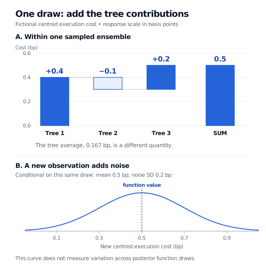
Original stipulated illustration, not fitted market data. Panel A sums component trees within one draw. Panel B adds observation noise conditional on that draw; it is not a posterior credible band for the conditional mean.
Why the trees stay small
The original regularising prior favours shallow trees and shrinks terminal-node values toward a common centre after response centring. This lets many weak components share the fit. “Additive” refers to addition of trees, not a ban on predictor interactions.
Bayesian backfitting repeatedly revisits a fixed collection of trees. To update tree , it forms partial residuals
then samples an update of that tree conditional on these residuals, the noise scale and the prior. The sampler also updates the noise scale. It revisits earlier components rather than permanently appending each tree as in gradient boosting. See the original paper, §§2.2–3.1.
Two different uncertainties
After burn-in, retained Markov chain Monte Carlo draws give different ensembles and hence values . Average those complete function draws for a posterior mean; use their quantiles for a pointwise credible interval. One ensemble draw cannot supply that interval. The official dbarts documentation distinguishes expected-value draws from posterior predictive draws.
A future observation requires an additional step:
If our single illustrative draw has bp squared, its noise standard deviation is bp. Conditional on that draw, a new centred cost has mean bp and variance bp squared. That variance is not the posterior variance of the function. Across the full posterior, the predictive variance combines both sources:
Here is the training data. This decomposition assumes the stated conditionally independent, mean-zero observation model. Financial cost noise may change with liquidity or have heavy tails; a constant Gaussian noise model does not capture those features merely by using flexible trees.
Prediction is the starting point
For execution-cost research, construct predictors using information available before the order decision. Fit response centring, preprocessing and prior calibration within each training window. Evaluate on later orders, handle overlapping outcome windows, and inspect predictive coverage across liquidity conditions. A narrow posterior interval under the fitted model does not account for an omitted regime change. The Finance-aware validation lesson develops overlap exclusions; its full teaching requires membership, with a public preview available.
A binary default outcome needs a suitable likelihood and link: the probit BART extension models , rather than treating the raw tree sum as a probability. See dbarts: numeric versus binary responses.
Nor does including an execution-policy indicator automatically identify its causal effect. An observational comparison still needs consistency, conditional exchangeability and overlap. Bayesian causal forests modify the response model and priors to separate prognostic effects from treatment-effect heterogeneity; they are a related extension, not another name for ordinary BART. See Hahn, Murray and Carvalho, §§2–3.
Sources
- Chipman, George and McCulloch (2010), BART: Bayesian additive regression trees, §§1–3.
- dbarts official R documentation: model, fitting and prediction types.
- Hahn, Murray and Carvalho, Bayesian regression tree models for causal inference: regularization, confounding, and heterogeneous effects, §§2–3.