The Bayes classifier minimises population misclassification under 0–1 loss. A two-state example explains the Bayes error rate, oracle knowledge and irreducible uncertainty.
Bayes-optimal classifier and Bayes error rate
A Bayes-optimal classifier chooses the label that minimises expected classification loss under the true data distribution, using the available features. Under 0–1 loss—zero for a correct label, one for a mistake—it predicts the most probable class. Its population misclassification probability is the Bayes error rate. For a quant forecasting a binary event, this separates errors that better learning might remove from uncertainty that remains even with perfect knowledge of the conditional probabilities. MIT's classification notes establish this population benchmark.
Why the majority label wins
Let Y∈{0,1} be the label, X the features and
η(x)=P(Y=1∣X=x).
At a fixed feature value, predicting 0 is wrong with probability η(x); predicting 1 is wrong with probability 1−η(x). Choosing the smaller conditional error gives
h∗(x)={1,0,η(x)>1/2,η(x)≤1/2.
Here a tie is assigned to class 0; either label has the same conditional risk when η(x)=1/2. Minimising separately at each x also minimises the average over X. This is a decision about a specified loss function: unequal mistake costs can change the optimal threshold. Chen's university notes derive the conditional-risk argument.
The resulting error floor is
R∗=P(h∗(X)=Y)=E[min{η(X),1−η(X)}].
For multiple classes under 0–1 loss, choose a class with maximal conditional probability; the error rate is one minus the expected largest class probability. Balakrishnan's classification review gives both forms.
Two feature states, four possible rules
Consider a fictional event label Y and a signal state X. Suppose A and B each occur with probability 0.5, with known conditional probabilities:
Feature state
Probability of label 1
Bayes prediction
Conditional error
A
0.70
1
0.30
B
0.20
0
0.20
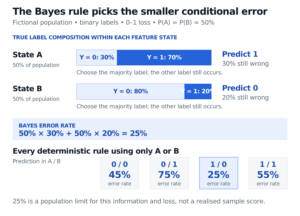
The Bayes error is 0.5(0.30)+0.5(0.20)=0.25. Always predicting 0 instead gives 0.5(0.70)+0.5(0.20)=0.45. Using the signal reduces population error by 20 percentage points.
The rule still misses 30% of A cases and 20% of B cases. Knowing a 70% event probability is different from knowing which individual events will occur.
Fictional binary population with equally likely states A and B. The positive-label probabilities are 70% and 20%. Predicting 1 in A and 0 in B gives conditional errors of 30% and 20% and a Bayes error of 25%; always predicting 0 gives 45% error.
Original finite-population illustration. Choosing the most likely label minimises mistakes but does not make the minority label disappear. All four deterministic rules using the two states are compared.
These are population probabilities, not promised frequencies in a finite test sample. A particular test sample can score above or below 25% error by chance.
What “irreducible” is relative to
The floor applies to the chosen information X, label definition and population distribution. If extra usable information distinguishes cases previously grouped together, the Bayes error can fall. A label determined completely by the available features has zero Bayes error; overlapping conditional label probabilities produce a positive floor. “Irreducible” therefore does not mean an immutable property of the event across every possible information set.
Changing the deployment distribution changes the benchmark too. In finance, information must be available when the forecast is made: adding tomorrow's outcome as a feature would change the mathematical problem while invalidating the forecast. Moreover, minimising the count of wrong direction forecasts does not optimise trading returns: magnitudes, costs and position choices enter a different objective.
An oracle benchmark, not a fitted model
The population rule assumes the true η is known. A learned classifier uses an estimate η^ or learns a boundary directly; thresholding estimated probabilities at one half does not prove Bayes optimality. Its population error may exceed R∗ because of limited data, model restrictions or estimation error. The true Bayes error generally cannot be read off from a training error or a single test score. MIT's discussion of the idealised classifier makes this distinction explicit.
The word “Bayes” also needs care. Bayesian inference updates uncertainty about unknown quantities using a prior and data. Bayes decision optimality concerns which action minimises expected loss given a probability law. The classifier above requires no prior over model parameters: P(Y∣X) is a class probability under the population law. A Bayesian posterior predictive distribution can supply class probabilities, but optimality under that model does not establish that it equals the true population law. Jordan’s decision-theory notes distinguish posterior expected loss, prior-averaged risk and the probabilities supplied by a Bayesian model.
For the fitted-model side, see Generative Classifiers. For decision thresholds and class-specific errors, see Evaluating Classifiers. Both have public previews; the full lessons require membership.