Bag of words represents a document by token counts, discarding word order. TF-IDF (term frequency–inverse document frequency) multiplies a within-document frequency by a weight that increases when the token appears in fewer documents. In financial research, this gives filings or news articles numerical features for retrieval, comparison or classification. A highly weighted word is distinctive within the chosen corpus; it need not express sentiment or predict returns.
Two different counts
Start with three fictional documents: D1 is “rate rises”, D2 is “rate falls”, and D3 is “bond yield”. Treat each complete string as one document. For this example, lowercase and extract contiguous ASCII letters
a through z. Keep single-word tokens, with no stemming, stop-word removal or frequency filtering. These are chosen conventions, not a universal text tokenisation rule.Fix the vocabulary columns in alphabetical order:
| Document | bond | falls | rate | rises | yield |
|---|---|---|---|---|---|
| D1: rate rises | 0 | 0 | 1 | 1 | 0 |
| D2: rate falls | 0 | 1 | 1 | 0 | 0 |
| D3: bond yield | 1 | 0 | 0 | 0 | 1 |
| Document frequency | 1 | 1 | 2 | 1 | 1 |
Term frequency (TF) here is the raw occurrence count in one document. Document frequency (df) counts documents containing the term at least once. Repeating “rate” several times inside D1 would raise its TF in D1, while D1 would still contribute only one to its df. Large document-feature tables are usually stored as a sparse matrix, because most documents contain only a small subset of the vocabulary.
One fully specified weighting rule
Use the current scikit-learn
TfidfTransformer convention with raw TF, natural logarithms, IDF smoothing enabled and L2 row normalisation. Before normalising, defineHere . Therefore
The other three words also appear in just one document and get the same IDF as “rises”. Both nonzero term counts in D1 are 1, so its unnormalised weights are exactly those two IDF values. Its Euclidean length is
Divide every component by that length. In the table's column order, D1 becomes
L2 normalisation gives a nonzero row unit Euclidean length. It removes uniform scale: doubling every token count in a document leaves its normalised vector unchanged under this raw-TF rule. It does not remove every difference associated with document length. The dot product of two nonzero L2-normalised rows is their cosine similarity, which compares feature directions rather than raw count totals. See the official TF-IDF API for the parameter definitions.
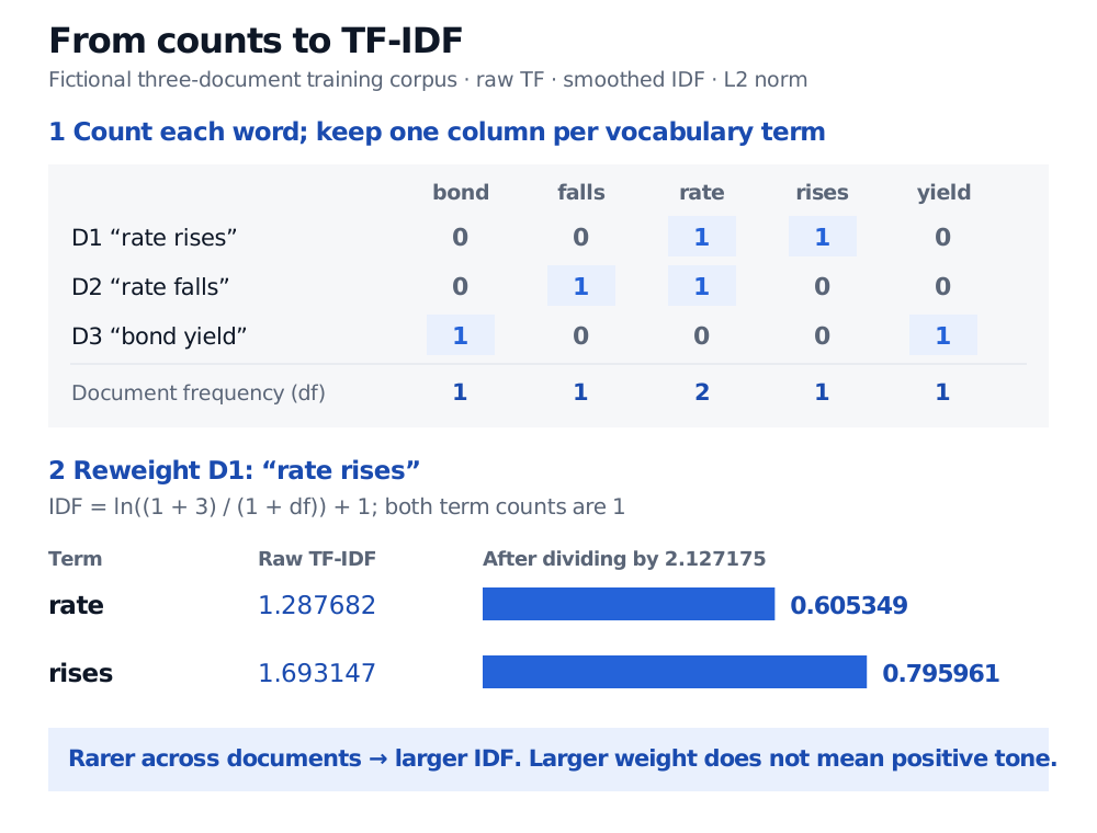
Original fictional corpus. Count occurrences within each document, count document presence across the corpus, then weight and normalise. The weighting rule measures rarity, not sentiment.
“TF-IDF” names a family of schemes. An unsmoothed rule assigns zero IDF to a word present in every document; the smoothed, offset rule above assigns it 1. Other schemes log the term counts or use different normalisation. Spärck Jones's original specificity argument motivates greater weight on rarer collection matches; it is not the exact software formula used here. Record the convention before comparing results.
What the vector cannot tell you
The unigram counts for “rates do not fall” and “rates fall not do” are identical. One is a normal sentence and the other is not; the representation cannot recover their order. Keeping “not” preserves its presence, but does not say which word it qualifies. Bigrams can retain adjacent pairs, while text embeddings provide a different representation. Neither choice establishes financial meaning by itself. The official text feature extraction guide discusses these representation limits.
For a forecasting evaluation, fit the vocabulary, frequency filters and IDF on the training documents only, then keep that fitted transformation fixed for the held-out period. Refit inside each training fold or dated training window. A fixed learned vocabulary ignores unseen tokens; a document with no retained tokens remains an all-zero row and has no defined cosine direction.
In a historical financial test, the training corpus must also respect the information cutoff: use document versions actually available then, with release and receipt delays accounted for. Computing df from later filings creates look-ahead bias even without using return labels. This applies the general training-only preprocessing rule to a dated corpus.
For a fuller treatment, Text Representation develops corpus and similarity choices. Finance-Specific Lexicons shows the additional step from word counts to a financial tone measure and uses a different term-weighting convention. Both have public previews; full lessons require membership. A useful retrieval representation still needs separate evidence before it can be treated as a return forecast.
Sources
- Karen Spärck Jones (1972), A statistical interpretation of term specificity and its application in retrieval, especially “Specificity and matching” and “Weighting by specificity”; author-hosted 2004 reprint.
- scikit-learn, Text feature extraction, especially bag of words, sparsity, TF-IDF and representation limitations.
- scikit-learn, TfidfTransformer, formula and TF, smoothing and normalisation parameters.
- scikit-learn, Data leakage, training-only preprocessing and cross-validation.