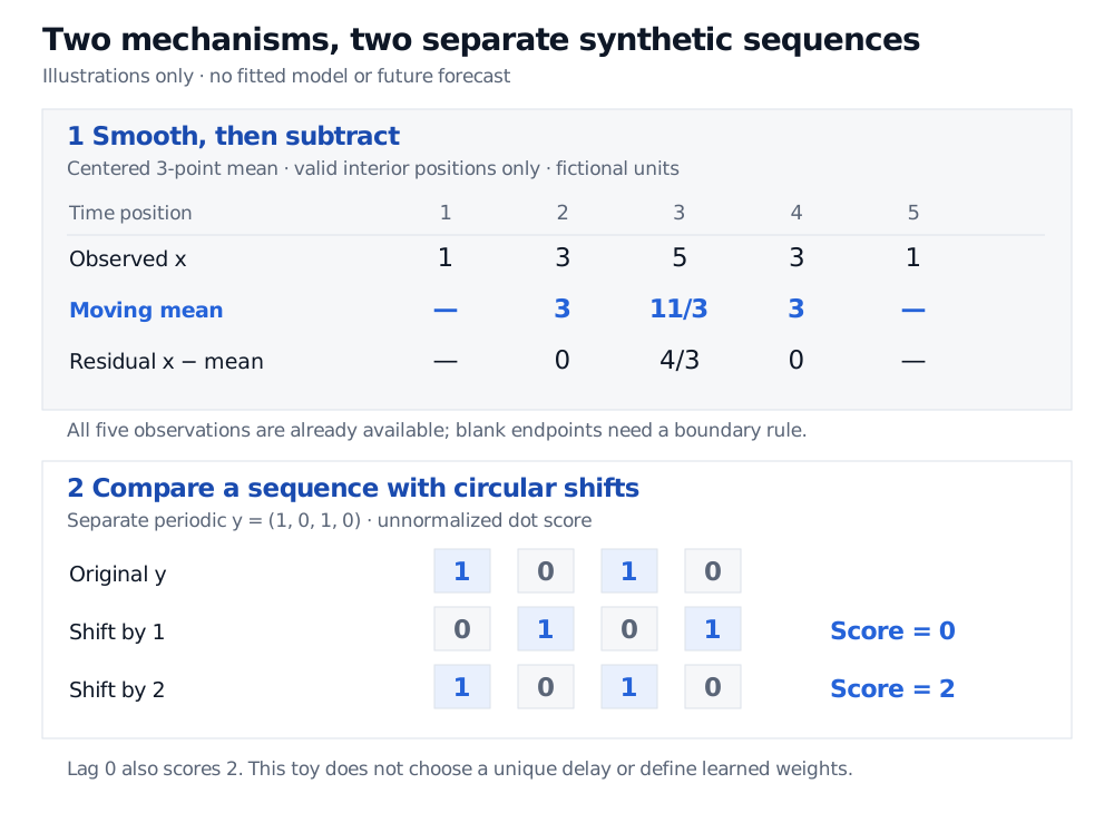
Autoformer combines progressive series decomposition with delay-based aggregation for long-horizon forecasting. Two small examples separate its smoothing and periodicity ideas from a learned financial forecast.
Autoformer
Autoformer is a neural architecture for long-horizon time-series forecasting that combines repeated decomposition of internal sequences with an Auto-Correlation mechanism that aggregates time-shifted subsequences. For a quant, it provides a way to model slow movements and recurring temporal structure jointly; using the architecture does not establish that a financial target is predictable. The original 2021 paper introduces both mechanisms.
Decomposition inside the model
A conventional workflow might decompose the observed series once, then forecast its components. Autoformer instead embeds decomposition throughout its encoder and decoder. A moving average extracts a trend-cyclical component; subtraction leaves what the paper calls a seasonal component. The decoder accumulates trend contributions while refining the remaining representation. These labels describe model components: the residual need not contain only seasonality, and smoothing does not prove stationarity. See §3.1.
To isolate the subtraction, take the fully observed, fictional sequence (1,3,5,3,1). At its three interior positions, use a centered three-point mean:
mt=3xt−1+xt+xt+1,rt=xt−mt.
Interior position
Observation
Moving mean
Residual
2
3
3
0
3
5
11/3
4/3
4
3
3
0
At the middle point, averaging 3,5,3 gives 11/3, so subtraction leaves 5−11/3=4/3. The components reconstruct the observations exactly at these positions; that identity says nothing about future forecast accuracy.
This toy omits endpoints. The authors’ decomposition code repeats the first and last values before average pooling, preserving sequence length. It applies decomposition to hidden sequences as well as the initial observations. A smoothing window is an architectural choice, not an automatically discovered economic trend.
The centered calculation here uses only an already available context window. Applying the same filter to an entire dataset before making historical train/test splits could instead let later observations enter earlier features. A centered filter at a historical position is not a forecast issued at that position.
Similarity across delays
Autoformer replaces ordinary point-to-point attention with delay-based aggregation. It scores alignments between projected query and key sequences, selects strong delays and combines shifted value sequences using softmax weights. FFT computation and a logarithmic number of selected delays give the mechanism its O(LlogL) sequence-length scaling, holding other dimensions fixed. See §3.2.
Use a separate periodic toy, y=(1,0,1,0), indexed from 0 to 3. Define the unnormalized circular dot score
C(τ)=t=0∑3yty(t−τ)mod4.
A shift by one produces (0,1,0,1), so every product is zero and C(1)=0. A shift by two restores (1,0,1,0), giving C(2)=1+0+1+0=2. The two-step repetition aligns the nonzero entries. Lag zero also scores 2: this toy alone does not select a unique delay.
Two separate synthetic toys: observations 1, 3, 5, 3, 1 have interior centered means 3, 11/3, 3 and residuals 0, 4/3, 0. Circular shifts of the separate sequence 1, 0, 1, 0 give unnormalized dot scores 0 at lag 1 and 2 at lag 2; lag 0 also scores 2.
Original mechanism illustrations in fictional units. Endpoint means are omitted in the first toy; the second deliberately wraps around. Neither panel is an Autoformer forecast or a learned hidden representation.
This is not a Pearson correlation coefficient: there is no demeaning or variance normalization, and circular wrapping differs from dropping unavailable lagged observations. The authors’ Auto-Correlation implementation computes FFT-based circular query–key scores, with learned projections and averaging across representation dimensions. Its faster training path shares the selected delay indices across a batch, while inference selects them per example. Softmax weights apply over selected delays; the score 2 above is neither a probability nor a forecast.
From mechanism to an honest forecasting experiment
The original model code initializes future seasonal slots with zeros and future trend slots with the observed context mean. The decoder refines these placeholders and adds the final seasonal and trend outputs. It does not fill them with realized future target values. Both toys above stop before these learned operations.
For financial use, define the target, sampling clock, horizon and information availability first. A lag measured in rows can change its economic meaning when trading sessions or missing observations change. Fit scaling and select the smoothing window and other settings within training/validation periods. Compare forecasts on the same later dates with simple baselines under a declared loss; if forecasts drive trades, separately assess turnover, costs and decision value. A recurring alignment in the training context may disappear after a regime change.
The SelfMadeQuant Forecast Evaluation lesson develops chronological experiments and loss comparisons. Its preview is public; the full lesson requires membership.