Appraisal smoothing is the dampening and delay of reported asset returns when appraisals reflect changes in market value gradually. It matters when comparing returns calculated from a private fund’s reported net asset value with returns on a portfolio priced in active markets. A smoother return series can make the private exposure look less volatile and less tied to the public market at the same reporting frequency. Geltner’s real-estate study.
A property can go years between sales. Its appraiser may rely on older comparable sales or reuse evidence that also informed the previous valuation. A fund can publish every quarter even when some marks carry forward or properties are reappraised on staggered dates. The same market news then feeds into several successive reports. The NCREIF Property Index uses appraisals to measure private commercial real estate returns and incorporates the actual sale price when a property sells. Fisher on appraisal timing, NCREIF methodology FAQ, NCREIF Trends Report.
One shock, several markdowns
Suppose a property starts at 100 and its unobserved market value drops to 80. For illustration, each quarter's appraisal mark moves 25% of the distance from its previous mark to the assumed market value . The rule acts on value levels, with no cash flows in the example.
The first mark is . That is a −5% reported price return against an assumed −20% market-value return. If market value stays at 80 in quarter 2, the mark falls again to 91.25. The second markdown reflects part of the first quarter’s shock. The 25% adjustment is a model input chosen to show the delay.
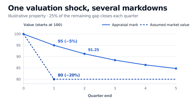
One valuation shock produces several quarters of markdowns when the appraisal closes only a quarter of the remaining gap at each update.
Reading a smooth track record
When successive reports share information about earlier shocks, the reported returns can show positive autocorrelation even if the underlying shocks are independent. In a smoothing model this can depress measured quarter-to-quarter volatility and inflate a positive Sharpe ratio. Comparing only same-quarter returns can also miss part of the exposure to a public benchmark if private marks respond in later quarters. Genuine persistence in economic returns can also produce autocorrelation. Getmansky, Lo and Makarov, sections 3–5, Geltner’s real-estate study.
An analyst can inspect when assets were reappraised, compare available sale prices with prior marks and look at how reported returns relate to current and lagged benchmark moves. A sale-price comparison needs both dates because the property's value can change between appraisal and sale. An unsmoothing model estimates how much of the reported change belongs to earlier periods. In the toy example, a mark of 95 implies a current value of 80 with a 25% adjustment but 90 with a 50% adjustment. The data point is the same. Any estimate of economic volatility from that exercise depends on the assumed adjustment rule and the quality of the marks. Geltner’s real-estate study.
The Backtest Evaluation lesson works through the covariance terms that affect Sharpe ratio annualisation when returns are correlated. The preview is public and the full lesson requires membership.
Sources
- David Geltner, Estimating Market Values from Appraised Values without Assuming an Efficient Market, working paper abstract (1992).
- Jeffrey D. Fisher, US commercial real estate indices: the NCREIF property index, BIS Papers (2005).
- Mila Getmansky, Andrew W. Lo and Igor Makarov, An Econometric Model of Serial Correlation and Illiquidity in Hedge Fund Returns (2003 author draft, published 2004).
- NCREIF methodology FAQ on the property and transaction-based indices and NPI Trends Report.