Measure a learning rule’s sensitivity to one training observation, distinguish uniform and averaged stability, and read its generalisation guarantee correctly.
Algorithmic stability
Algorithmic stability measures how much a learning procedure's predictions or losses change when its training sample is perturbed. For a quant researcher, it asks whether a fitted signal depends heavily on particular observations. Under suitable sampling assumptions, controlling that sensitivity also controls the gap between training loss and generalisation error.
The object is the whole learning rule, including any fitted preprocessing and model selection being analysed. It is not a claim that markets, prices or portfolio returns are stable, and it differs from the numerical stability of floating-point computations.
Change one observation, keep the test point fixed
Let A(S) be the predictor fitted to a sample S of size n, and let ℓ(A(S),z) be its loss on a test observation z. Here, a deterministic learner has uniform replace-one stabilityβn if
S,S′,zsup∣ℓ(A(S),z)−ℓ(A(S′),z)∣≤βn,
where S and S′ differ in at most one observation. “Uniform” means every allowed neighbouring pair and every allowed test point. Loss units and the allowed data domain are part of the statement. Hardt, Recht and Singer, §2, use the replace-one convention, allowing randomised algorithms through expectation over their internal randomness.
A mean learner with a sharp bound
Consider a fictional learner with bounded scalar observations yi∈0,1]. It predicts their [sample mean for every new observation and is assessed using absolute loss:
A(S)=yˉ=n1i=1∑nyi,ℓ(yˉ,y)=∣yˉ−y∣.
Replacing yi by yi′ changes the prediction by
∣yˉ−yˉ′∣=n∣yi−yi′∣≤n1.
The reverse triangle inequality then controls the loss at the same test outcome:
∣∣yˉ−y∣−∣yˉ′−y∣∣≤∣yˉ−yˉ′∣≤n1.
This is a proof over the full bounded domain, not an inference from a few successful refits.
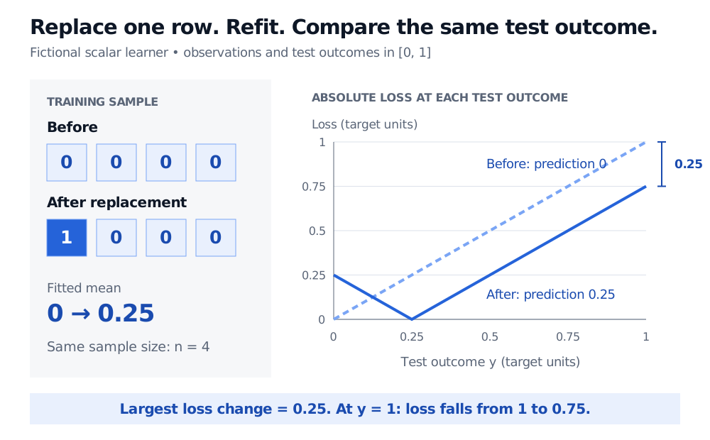
For n=4, start with four zeros and replace one zero by one. The fitted mean moves from 0 to 1/4. At test outcome y=1, absolute loss falls from 1 to 3/4: a change of exactly 1/4. Thus the uniform bound β4=1/4 is attained. At y=1/8, both losses equal 1/8; the bound does not say every test loss changes by the maximum.
Fictional bounded mean learner: replacing one zero by one among four observations changes its prediction from 0 to 0.25. Absolute-loss curves differ by at most 0.25 on test outcomes from 0 to 1; at outcome 1, losses are 1 and 0.75.
Original fictional scalar example. Dashed and solid curves show absolute loss before and after replacement; both use the same test outcome and target units.
Bounding the observations is essential to this particular 1/n result. Unbounded replacements can move the sample mean arbitrarily far. Another learner, loss or preprocessing rule needs its own analysis.
Why deletion and averages change the claim
Bousquet and Elisseeff's original paper, §3, defines uniform stability using deletion: compare training on S with training on S minus one observation. Their deletion bound β implies a replace-one bound 2β by comparing both full samples with their common reduced sample. A quoted constant therefore needs its perturbation convention.
Their hypothesis stability instead averages the absolute loss change over the random training sample and an independent test observation, for each deleted index. It can hide exceptional samples or test points that a uniform bound must cover. “On-average stability” also needs its precise definition: specify what is averaged, whether an absolute value is inside the expectation, and whether the comparison uses a fresh or a training observation. These are not interchangeable guarantees.
Deletion is also the operation behind leave-one-out cross-validation. An observed leave-one-out score estimates predictive error; it does not prove a worst-case stability bound.
What stability buys—and what it leaves open
For a measurable deterministic learner with the replace-one bound above, suppose the training observations are independent and identically distributed from D, and a fresh test observation independently follows the same D. Assume the losses are integrable. Define
This is the deterministic case of Hardt, Recht and Singer's Theorem 2.2. The absolute value is outside the expectation. It neither bounds the expected absolute gap by the same constant nor gives a high-probability guarantee for one fitted sample. The bounded mean example satisfies the integrability condition when test outcomes also lie in [0,1].
A small gap can coexist with poor prediction: a learner that always outputs zero has zero replacement sensitivity, yet absolute loss one when every outcome is one. Stability controls sensitivity and, under the theorem's assumptions, average optimism; it does not establish useful forecasts.
In financial research, refitting after removing observations or blocks can reveal concentration of influence. Such diagnostics do not establish the uniform supremum. Serial dependence, overlapping labels and distribution shifts also prevent automatic use of the i.i.d. theorem. Time-Ordered Train, Validation and Test Design develops the information boundaries and refitting schedule needed for forecasting evaluation (full lesson requires membership; public preview available). Stability analysis complements that evaluation; it does not certify future trading performance.
Sources
Bousquet, O. and Elisseeff, A. (2002), Stability and Generalization, Journal of Machine Learning Research 2, 499–526; §2.1, Definitions 3–6 and Lemma 7: sampling setup, deletion-based criteria and the replace-one bridge.