Adaptive lasso: Definition & Examples

Adaptive lasso is a weighted version of Lasso regression whose coefficient penalties are determined by an initial, or pilot, estimate. A quant screening candidate return predictors can penalise small pilot coefficients more heavily while shrinking large ones less. The resulting feature selection remains conditional on the model and data; it does not identify economic causes.

A pilot changes the price of each coefficient

For centred data, let $y$ be the response vector and $X$ the predictor matrix. With a nonzero pilot coefficient $\widetilde\beta_j$ , set

w_j=\frac{1}{\lvert\widetilde\beta_j\rvert^\gamma}, \qquad \gamma>0, \qquad \widehat\beta =\operatorname*{arg\,min}_\beta \left\{\frac12\lVert y-X\beta\rVert_2^2 +\lambda\sum_{j=1}^p w_j\lvert\beta_j\rvert\right\}, \qquad\lambda\geq0.

The weights are fixed during this second fit. Its objective is convex. A separately fitted intercept is normally unpenalised. Zou (2006), §3.1.

This page uses unaveraged half squared error. If software instead uses

\lVert y-X\beta\rVert_2^2/(2n)+\alpha\sum_jw_j\lvert\beta_j\rvert

, the equivalent parameter is

\alpha=\lambda/n

, holding weights fixed. If the loss is the full squared error without the half, double this page's penalty parameter. Comparing numerical penalties without their loss convention is misleading.

A zero pilot needs an explicit policy: the reciprocal is undefined. Treating its weight as infinite at positive $\lambda$ forces that coefficient to zero permanently. A positive floor such as $w_j=(\lvert\widetilde\beta_j\rvert+\varepsilon)^{-\gamma}$ avoids infinity but changes the estimator. A ridge pilot can reduce instability from collinearity; no pilot choice automatically supplies the original theorem's assumptions.

Two predictors, two thresholds

Consider a synthetic, dimensionless example with centred, mutually orthogonal, unit-norm predictor columns:

X^\top X=I

. The ordinary least squares coefficients are

z=X^\top y=(3,0.5)^\top

. Supply an illustrative nonzero pilot

(2,0.5)^\top

, obtained without test outcomes. It is an input to this example, not the OLS fit just stated.

Take $\gamma=1$ and $\lambda=1$ . The weights are $(0.5,2)^\top$ . Expanding the squared error and dropping its constant leaves separate scalar objectives:

\frac12(\beta_j-z_j)^2+\lambda w_j\lvert\beta_j\rvert.

For a positive solution, differentiation gives $\beta_j=z_j-\lambda w_j$ ; the negative branch is symmetric, and zero is optimal between the two thresholds. Thus

\widehat\beta_j =\operatorname{sgn}(z_j)\max(\lvert z_j\rvert-\lambda w_j,0).

Predictor	OLS coefficient	Pilot	Weight	Threshold	Adaptive estimate
1	3	2	0.5	0.5	2.5
2	0.5	0.5	2	2	0

Ordinary lasso with unit weights and the same loss and $\lambda$ gives $(2,0)^\top$ . Here adaptation reduces shrinkage of the first coefficient. It provides no evidence that this predictor forecasts better. With correlated columns, the scalar problems no longer separate; thresholding marginal OLS coefficients is not the adaptive-lasso solution.

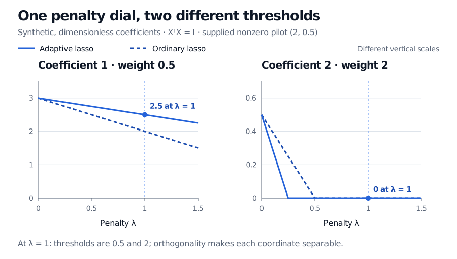
Synthetic orthonormal-design coefficient paths. At penalty 1, adaptive weights 0.5 and 2 give coefficients 2.5 and 0; ordinary lasso gives 2 and 0. The coefficient panels use different vertical scales.

Original illustrative calculation with fixed pilot coefficients (2, 0.5). Solid lines use adaptive weights; dashed lines use unit weights. These paths show shrinkage, not forecast performance.

What must stay inside training

The pilot is a learned step. In cross-validation, refit scaling, pilot estimation, weights and the weighted regression inside each training fold, including inner folds used to tune the procedure. A full-history pilot leaks held-out outcomes even if the second fit uses only training rows. This applies the official leakage guidance to the complete two-stage estimator. For return forecasts, preserve time order and use only labels available at the fit cutoff.

Document the feature scale for both stages. Under $x'_j=cx_j$ with $c>0$ , a scale-equivariant pilot transforms to $\widetilde\beta'_j=\widetilde\beta_j/c$ . The penalty contribution then changes by $c^{\gamma-1}$ . The special case $\gamma=1$ is invariant under that ideal transformation; a ridge pilot or an absolute pilot floor can break it. Standardising from training data gives a reproducible convention, but does not make columns orthogonal.

“Oracle” is an asymptotic statement

Zou's Theorem 2 establishes consistent support recovery and oracle-limit coefficient variance in a fixed-dimensional linear model with iid zero-mean, finite-variance errors, a positive-definite limiting design Gram matrix, a root-

n

consistent pilot and suitable tuning rates. Under this page's half-loss convention, the rates remain

\lambda_n/\sqrt n\to0

and

\lambda_n n^{(\gamma-1)/2}\to\infty

Those conditions do not promise correct finite-sample selections, causal truth, or validity for an arbitrary high-dimensional or dependent-return problem. Prediction-based tuning alone does not certify them. Nor does adaptive weighting itself produce selection-adjusted confidence intervals; that is a separate post-selection inference problem.

For the ordinary-penalty foundation and correlated-predictor intuition, see Ridge, Lasso, and Elastic Net (public preview; full lesson requires membership).

Sources

Zou, H. (2006), The Adaptive Lasso and Its Oracle Properties, JASA 101(476), 1418–1429: §2 assumptions; §§3.1–3.2 construction and oracle result; §3.5 pilot and tuning choices. The paper's main regression objective uses full squared error; this page explicitly rescales it.
scikit-learn, Common pitfalls and recommended practices, data leakage during preprocessing: fitting learned transformations within the appropriate training subsets.

A pilot changes the price of each coefficient

Two predictors, two thresholds

What must stay inside training

“Oracle” is an asymptotic statement

Sources

Related terms

Debiased Lasso and post-selection inference

Feature selection

Ordinary least squares