AdaGrad and RMSProp: Definition & Examples

AdaGrad and RMSProp are adaptive gradient descent methods that divide each parameter's current gradient by a scale built from its past squared gradients. AdaGrad retains the entire history; RMSProp discounts older observations. When fitting a financial prediction model, this gives different weights different effective learning rates without specifying a separate rate for every weight.

One learning rate, different denominators

Let

g_{t,i}

be the gradient of the training loss function with respect to parameter

i

, evaluated before update

t

. For the unconstrained, diagonal form of AdaGrad, start with

G_{0,i}=0

and use

G_{t,i}=G_{t-1,i}+g_{t,i}^2, \qquad \theta_{t,i}=\theta_{t-1,i}-\eta\frac{g_{t,i}}{\sqrt{G_{t,i}}+\epsilon}.

Here

\eta>0

is the base learning rate and

\epsilon>0

stabilises division. The accumulator is a sum of squares, not an average. A coordinate with more accumulated squared-gradient activity receives a smaller multiplier on its current gradient. This motivates AdaGrad for sparse features: an infrequently active coordinate need not inherit the smaller multiplier of a frequently active one. That comparison concerns gradient history, not a guarantee that a rare feature is informative. The original AdaGrad paper develops both diagonal and full-matrix methods; the formula here is the simpler diagonal case without constraints or a separate regularisation term.

RMSProp replaces the running total with an exponentially weighted average:

v_{t,i}=\rho v_{t-1,i}+(1-\rho)g_{t,i}^2, \qquad \theta_{t,i}=\theta_{t-1,i}-\eta\frac{g_{t,i}}{\sqrt{v_{t,i}}+\epsilon},

with

v_{0,i}=0

and

0\leq\rho<1

. The variant here is uncentred, without momentum or bias correction. It tracks squared-gradient scale rather than variance: no squared mean is subtracted. Hinton's Lecture 6, crediting Tijmen Tieleman, introduces this moving-average division.

Both formulas place epsilon outside the square root. This matches the documented PyTorch Adagrad update with learning-rate decay and weight decay disabled, and PyTorch RMSprop with centering, momentum and weight decay disabled, checked 1 November 2026. An implementation using

\sqrt{v+\epsilon}

has a different denominator from

\sqrt v+\epsilon

. Check the formula and initial accumulator, rather than matching parameter names alone.

Two unchanged gradients, four different moves

Consider a stipulated scalar gradient sequence

g_1=g_2=2

, base learning rate

\eta=0.1

and RMSProp decay

\rho=0.9

. Set

\epsilon=0

only for this analytic toy: every accumulator used in a divisor is positive. Practical implementations use positive epsilon, including when a coordinate's gradient history is zero.

Update	AdaGrad accumulator	AdaGrad step magnitude	RMSProp accumulator	RMSProp step magnitude
1	$4$	$0.1000000000$	$0.4$	$0.3162277660$
2	$8$	$0.0707106781$	$0.76$	$0.2294157339$

For example, the second RMSProp average is $0.9(0.4)+0.1(4)=0.76$ , giving a step magnitude of $0.1(2)/\sqrt{0.76}$ . Since the gradients are positive, each update subtracts the listed amount from the parameter. These are prescribed observations, not a simulated loss trajectory or a benchmark.

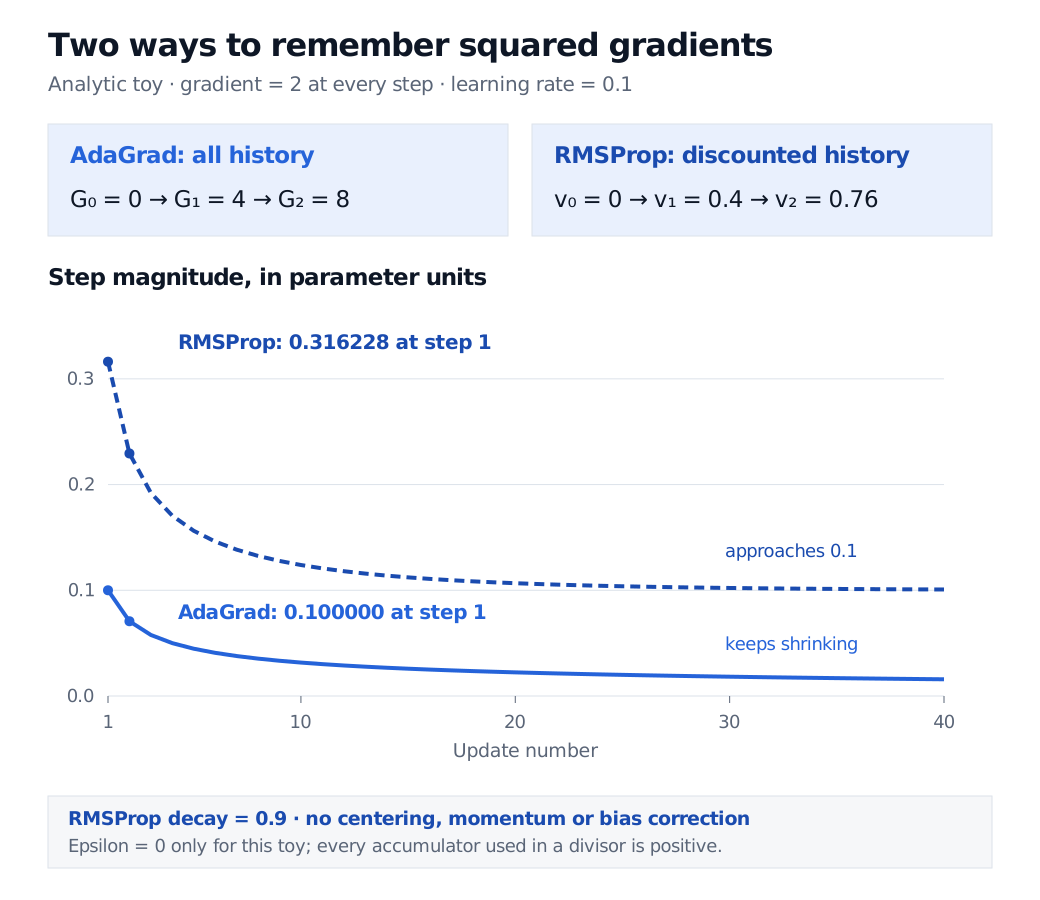
Analytic toy with gradient 2 and learning rate 0.1: AdaGrad accumulators 4 and 8 give steps 0.100000 and 0.070711; uncorrected RMSProp accumulators 0.4 and 0.76 give steps 0.316228 and 0.229416. With the gradient held constant, AdaGrad steps keep shrinking while RMSProp steps approach 0.1.

Identical incoming gradients produce different steps because the denominators remember different histories. The large early RMSProp steps reflect its zero-initialised average, not evidence of better optimisation.

Holding that nonzero gradient constant gives exact expressions:

G_t=4t,\qquad v_t=4(1-\rho^t),\qquad \lvert\Delta\theta_t^{\mathrm{AdaGrad}}\rvert=\frac{0.1}{\sqrt t},\qquad \lvert\Delta\theta_t^{\mathrm{RMSProp}}\rvert=\frac{0.1}{\sqrt{1-\rho^t}}.

AdaGrad's steps shrink indefinitely in this example. RMSProp's approach

0.1

from above as its zero-initialised average fills. Its early squared-gradient average is below its long-run value, making the denominator smaller; that initialisation transient explains the larger early moves. No correction factor is applied in this RMSProp variant. Adam adds signed gradient memory and moment corrections and is a separate algorithm.

What forgetting buys—and what it cannot decide

With fixed

\eta

, AdaGrad's effective multiplier cannot increase because its accumulator cannot decrease. The multiplier tends to zero if the cumulative squared gradients diverge; monotonic accumulation alone does not establish that limit. A large early gradient remains in its denominator permanently.

RMSProp gives a squared gradient observed $k$ updates ago a weight proportional to $\rho^k$ . Old large observations can therefore lose influence, allowing the multiplier to increase again. This adapts to changes in gradients during fitting; it does not establish that the method can handle a change in the market's predictive relationships.

Neither method averages signed gradients in the numerator in the forms shown here. That is the separate role of momentum. Neither removes the choice of base learning rate, decay, feature scaling or stopping rule, and neither is universally best. Compare training behaviour and chronological validation on the actual modelling task. The optimisation-choices lesson extends the recurrence comparison to SGD, momentum and Adam; its preview is public and the full lesson requires membership.

Sources

Duchi, Hazan and Singer (2011), Adaptive Subgradient Methods for Online Learning and Stochastic Optimization, Section 1.1, Equation 1 and Section 3's diagonal algorithm.
Hinton, Neural Networks for Machine Learning, Lecture 6, slide 29: RMSProp's squared-gradient moving average and Tieleman attribution.
PyTorch 2.15, Adagrad and RMSprop, update algorithms, initialisation and epsilon convention; checked 1 November 2026.

One learning rate, different denominators

Two unchanged gradients, four different moves

What forgetting buys—and what it cannot decide

Sources

Related terms

Adam optimiser

Loss function

Momentum and Nesterov acceleration