Momentum and Nesterov acceleration: Definition & Examples

Momentum is an optimisation method that carries information from earlier gradients into the next parameter update. It extends gradient descent: a parameter moves according to accumulated gradient history rather than the current gradient alone. For a quant fitting a volatility forecaster, this changes the training path and makes the saved optimiser state part of a reproducible experiment. It is separate from a trading strategy that buys recent market winners.

What the buffer remembers

Let

\theta_{t-1}

be the parameter vector before update

t

, and let

g_t

be the gradient of the training loss function at that point, possibly estimated from a mini-batch. One classical momentum convention is

v_t=\beta v_{t-1}+g_t, \qquad \theta_t=\theta_{t-1}-\eta v_t,

where

v_0=0

0\leq\beta<1

and

\eta>0

. Here

v_t

is a gradient buffer, with the learning rate applied outside it. This is the undampened momentum form documented by PyTorch SGD, with weight decay and Nesterov disabled.

Expanding the recurrence shows precisely what “memory” means:

v_t=g_t+\beta g_{t-1}+\beta^2g_{t-2}+\cdots+\beta^{t-1}g_1.

Gradients pointing in a similar direction reinforce one another. Opposing contributions partly cancel. The buffer does not know whether a direction is economically useful; it remembers gradients of the chosen training objective.

Take an illustrative scalar parameter with $\theta_0=1$ , $\beta=0.9$ , $\eta=0.1$ , and two stipulated gradient observations, $g_1=g_2=2$ .

Update	Buffer calculation	Parameter after update
1	$v_1=2$	$\theta_1=1-0.1(2)=0.8$
2	$v_2=0.9(2)+2=3.8$	$\theta_2=0.8-0.1(3.8)=0.42$

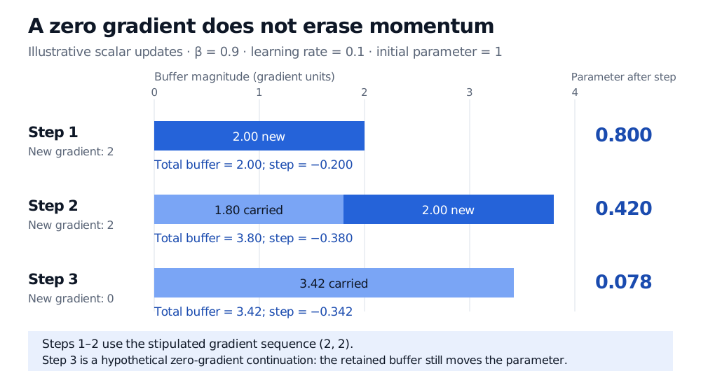
The second move has magnitude $0.38$ , even though the fresh gradient is unchanged. These are stipulated gradients, not a claim that every loss produces that sequence. If the next gradient were zero, the buffer would still be $v_3=3.42$ , moving the parameter to $0.078$ . A zero current gradient does not immediately stop an optimiser with nonzero memory.

Illustrative scalar momentum updates. Gradients 2 and 2 produce buffers 2 and 3.8 and parameters 0.8 and 0.42. A hypothetical third gradient of zero retains a buffer of 3.42 and moves the parameter to 0.078.

Carried gradient history and the new observation contribute separately to each buffer. The third step illustrates retained motion after the current gradient becomes zero.

A learning rate needs its convention

Another convention uses an exponential moving average:

m_t=\beta m_{t-1}+(1-\beta)g_t.

With both buffers initially zero and the same constant $\beta$ , algebra gives $m_t=(1-\beta)v_t$ . To reproduce the preceding parameter updates using $\theta_t=\theta_{t-1}-\eta_{\mathrm{EMA}}m_t$ , set

\eta_{\mathrm{EMA}}=\frac{\eta}{1-\beta}.

Thus the example's raw-buffer learning rate of $0.1$ corresponds to an EMA-buffer learning rate of $1$ . Copying the same numerical learning rate between these formulas changes the algorithm's step sizes.

There is another distinction: some implementations store the signed parameter displacement,

d_t=\beta d_{t-1}-\eta g_t

, then add it to the parameter. With a constant learning rate,

d_t=-\eta v_t

translates between these two forms. If the learning rate changes, old gradients in the displacement state retain their earlier learning-rate scaling; the raw-buffer form scales the whole current buffer by the new learning rate. PyTorch's implementation note explicitly distinguishes these conventions. Record the update rule, schedule and state initialisation when comparing implementations.

Nesterov moves the point where you ask for a gradient

In the signed-displacement notation, a lookahead form of Nesterov accelerated gradient is

\begin{aligned} y_t&=\theta_{t-1}+\beta d_{t-1},\\ d_t&=\beta d_{t-1}-\eta\nabla L(y_t),\\ \theta_t&=\theta_{t-1}+d_t. \end{aligned}

Classical momentum evaluates the gradient at

\theta_{t-1}

; Nesterov evaluates it at the projected point

y_t

. The lookahead lets the gradient correction respond to where the retained motion is taking the parameter. This is the formulation in Sutskever and co-authors, Section 2; framework parameterisations must be checked before equating their stored states.

A separate toy loss makes the difference visible. For $L(\theta)=\theta^2/2$ , start at $1$ with zero displacement, learning rate $0.1$ and momentum $0.9$ . Both methods first reach $0.9$ , with displacement $-0.1$ . On update two, classical momentum reads the gradient $0.9$ and reaches $0.72$ . Nesterov reads the gradient at $0.9+0.9(-0.1)=0.81$ and reaches $0.729$ . The methods already differ after two updates; this short example is not a performance ranking.

Faster fitting is a claim to test

Polyak's original two-step analysis explains the appeal of inertia in poorly conditioned problems, while also noting that the objective need not decrease on every iteration. Its nonlinear convergence results are local, under stated assumptions. See Polyak, Sections 1–2. Those results do not guarantee acceleration for an arbitrary nonconvex market model or convergence to its global optimum.

For a financial prediction experiment, tune learning rate and momentum together, preserve chronological validation, and compare validation performance as well as training loss. More rapid loss reduction alone does not establish a better trading signal or a particular explanation about the shape of the fitted minimum. The loss-curve diagnosis lesson develops experiment logging and model-selection discipline; its preview is public and the full lesson requires membership. Adam adds adaptive coordinate scaling to gradient memory, so it is a further method rather than another name for classical momentum.

Sources

Polyak (1964), Some methods of speeding up the convergence of iteration methods, Sections 1–2: local nonlinear results, two-step method and nonmonotone objectives.
Sutskever, Martens, Dahl and Hinton (2013), On the importance of initialization and momentum in deep learning, Sections 2–2.1: classical momentum and the Nesterov lookahead formulation.
PyTorch 2.15, SGD, algorithm and implementation note; checked 1 November 2026.

What the buffer remembers

A learning rate needs its convention

Nesterov moves the point where you ask for a gradient

Faster fitting is a claim to test

Sources

Related terms

Adam optimiser

Loss function