Sharpness-aware minimisation: Definition & Examples

Sharpness-aware minimisation (SAM) is a training method that seeks model weights with low loss throughout a small surrounding neighbourhood. It probes an uphill direction in weight space, then uses the gradient at that perturbed point for the learning update. For a quant fitting a neural return or volatility model, this changes the training objective and computational budget; an improvement still has to survive chronological validation.

The neighbourhood is part of the objective

For empirical loss

L(w)

and radius

\rho

, the core objective is

\min_w F_\rho(w), \qquad F_\rho(w)=\max_{\lVert\epsilon\rVert_2\le\rho}L(w+\epsilon).

The Euclidean ball constrains the joint length of the weight perturbation. It does not give every weight an independent allowance of

\rho

. The increase

F_\rho(w)-L(w)

measures local sharpness under this chosen norm and radius. Minimising

F_\rho

balances low loss with insensitivity to nearby weight changes; minimising sharpness alone could favour a flat region with high loss. A weight penalty may be added separately, as in Foret et al.'s formulation.

The practical step uses two gradients

For one mini-batch loss $L_B$ , the usual first-order, Euclidean SAM step is

\begin{aligned} g &= \nabla L_B(w), \\ \hat\epsilon &= \rho\frac{g}{\lVert g\rVert_2}, \\ \tilde g &= \left.\nabla_u L_B(u)\right|_{u=w+\hat\epsilon}, \\ w_{\mathrm{next}} &= w-\eta\tilde g. \end{aligned}

Here

g\ne0

and

\eta

is the learning rate; the last line uses plain gradient descent. Another base optimiser, such as Adam, can consume

\tilde g

instead.

Two approximations matter. The normalised gradient maximises a linearised loss, not the general nonlinear inner problem. The second gradient treats

\hat\epsilon

as fixed: it does not differentiate through the calculation of the perturbation. This is the stop-gradient, first-order procedure in the paper's Equation 3 and Algorithm 1. Differentiating through the approximate perturbation gives a different procedure with second-order terms.

The basic version uses the same mini-batch twice. Restore the original weights before applying the optimiser step. Its two forward/backward evaluations cost more than an ordinary update; elapsed time need not be exactly doubled. The authors' research repository provides the original experimental setting and code, rather than evidence about financial prediction.

A probe is not a permanent uphill update

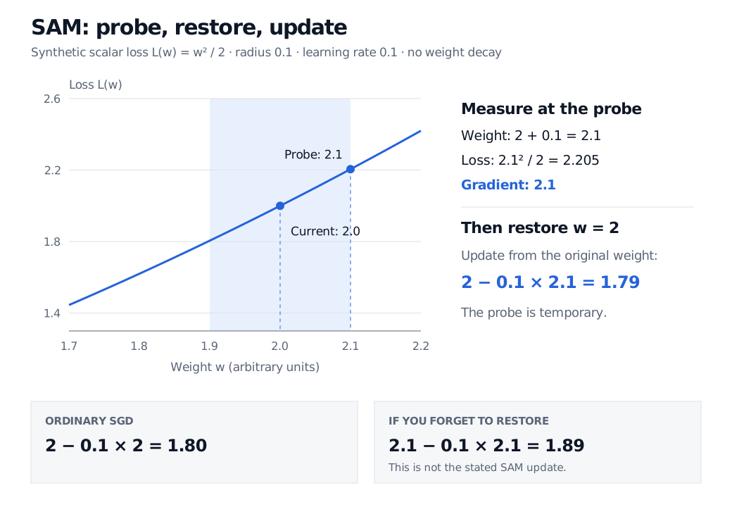
Take the synthetic scalar loss $L(w)=w^2/2$ , with current weight $w=2$ , radius $\rho=0.1$ , learning rate $\eta=0.1$ and no weight decay.

Operation	Result
Gradient at the current weight	$g=2$
Normalised uphill perturbation	$\hat\epsilon=0.1$
Probe weight and loss	$2.1$ and $2.205$
Gradient measured at the probe	$\tilde g=2.1$
Restore, then update	$2-0.1(2.1)=1.79$
Ordinary SGD from the same weight	$2-0.1(2)=1.80$

Synthetic quadratic loss: from w = 2, probe the radius-0.1 neighbourhood at w = 2.1, where loss is 2.205 and gradient is 2.1. Restore w = 2 before the update to 1.79; ordinary SGD would give 1.80.

The uphill probe chooses where to measure the gradient. The learning update starts from the original weight, not the perturbed weight. Synthetic scalar example; no weight decay.

Starting the final update from $2.1$ would instead give $1.89$ , which is not this SAM step. The probe temporarily increases the loss so the algorithm can measure a gradient there.

For this quadratic at positive $w$ , the exact neighbourhood maximum is at $w+\rho$ , so the approximate probe happens to find it. That coincidence is not a general property of neural-network losses. Even this quadratic exposes a limit at $w=0$ : the current gradient vanishes, yet the radius- $0.1$ neighbourhood contains loss $0.005$ . The normalisation formula is then undefined. Choosing a zero perturbation handles the division but misses that increase; it does not solve the inner maximisation.

Flatness needs a coordinate system—and a test

A flat-looking minimum is not a certificate of generalisation. Dinh et al. show that rescaling layers in rectified networks can preserve the prediction function while changing common sharpness measures. A fixed Euclidean radius therefore has meaning only relative to the parameterisation and scale. SAM's weight-space neighbourhood is also different from perturbing input features or market scenarios.

When comparing a financial model trained with SAM against its base optimiser, hold the data construction and chronological splits fixed, tune on validation, and record the radius, learning rate, weight-decay convention, seeds and compute budget. Report both predictive performance and training cost. Lower validation error alone does not establish that flatness caused the improvement; matching training losses does not establish that mechanism either. Weight robustness cannot repair future-data leakage or guarantee stability under a market-regime change.

Reading Loss Curves develops experiment logging, validation-based selection and training diagnosis. Its preview is public; the full lesson requires membership.

Sources

Foret, P., Kleiner, A., Mobahi, H. and Neyshabur, B. (2021), Sharpness-Aware Minimization for Efficiently Improving Generalization, Section 2, Equations 1–3 and Algorithm 1; Section 3.1 for evaluation cost.
Dinh, L., Pascanu, R., Bengio, S. and Bengio, Y. (2017), Sharp Minima Can Generalize For Deep Nets, Sections 3–4 on equivalent rectified networks and sharpness.
Google Research, SAM research repository, README: experimental scope and training configuration; accessed 1 November 2026.

The neighbourhood is part of the objective

The practical step uses two gradients

A probe is not a permanent uphill update

Flatness needs a coordinate system—and a test

Sources

Related terms

Adam optimiser

Generalisation

Loss function