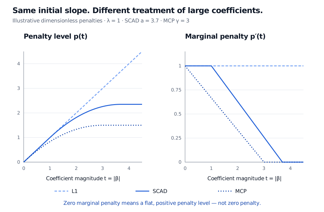
SCAD and MCP encourage sparse regression while tapering the penalty on large coefficients. Compare their slopes, penalty levels and optimisation limits.
SCAD and MCP regularisation penalties
SCAD (smoothly clipped absolute deviation) and MCP (minimax concave penalty) are coefficient penalties that encourage sparse regression while reducing the marginal penalty on large coefficients. In a return-prediction model with many candidate signals, they offer a way to discard weak predictors without applying the lasso's constant shrinkage pressure to every surviving coefficient.
Their distinctive feature is a penalty that eventually becomes flat. That changes estimation and optimisation; it does not establish which predictors cause returns.
Read the slope before the penalty level
For centred data, use the convention
Q(β)=2n1∥y−Xβ∥22+j=1∑ppλ(∣βj∣).
The intercept is excluded from the penalty. Predictor scaling matters because the same coefficient magnitude must have a comparable meaning across columns. The value of λ also depends on this loss normalisation.
Write t=∣βj∣≥0. Define each penalty by pλ(0)=0 and its derivative with respect to magnitude for t>0:
MCP starts tapering immediately. Zhang (2010), §2.1 defines it by integrating this slope; γ>1 is the convention used here, within the paper's broader family. Both penalties satisfy pλ′(0+)=λ. As functions of the signed coefficient, pλ(∣β∣) has a kink at zero. Away from zero its derivative is pλ′(∣β∣)sgn(β).
A slope of zero does not mean a penalty of zero
Set λ=1, a=3.7 and γ=3. These are illustrative dimensionless settings, not a tuning recommendation.
Coefficient magnitude t
SCAD marginal penalty
MCP marginal penalty
0.5
1
5/6≈0.8333
2
1.7/2.7≈0.6296
1/3≈0.3333
4
0
0
These entries are derivatives, not penalty values or fitted coefficients. For instance, at t=4 the penalty levels are SCAD: 2.35 and MCP: 1.5, obtained by integrating their slopes from zero. Both are positive but flat: increasing the magnitude further adds no penalty. L1 instead keeps adding λ per unit of magnitude.
With lambda 1, SCAD a 3.7 and MCP gamma 3, SCAD and MCP penalty levels plateau at 2.35 and 1.5. Their marginal penalties reach zero at coefficient magnitudes 3.7 and 3, whereas L1 has slope 1 throughout.
Illustrative dimensionless penalty levels and their slopes. A flat positive penalty contributes no additional cost when a sufficiently large coefficient increases.
Reduced marginal pressure can reduce shrinkage of large fitted coefficients. It does not make them accurate: sampling noise, correlated signals and model misspecification still affect the fit.
Nonconvex penalty, sometimes convex objective
The signed penalties are nonconvex. The whole penalised objective need not be: sufficient least-squares curvature can offset the penalty's negative curvature. For this normalisation, a sufficient condition for strict convexity is that the smallest eigenvalue of X⊤X/n exceeds 1/(a−1) for SCAD, or 1/γ for MCP. This follows by bounding the negative curvature of each penalty; Zhang's §2.1 distinguishes global curvature from curvature restricted to sparse models.
When that compensation is absent, several local solutions may exist. A solver's convergence to a stationary point does not certify a global minimum. Record the loss scaling, tuning parameters, initialisation and convergence criteria; compare solutions when optimisation is uncertain.
Fan and Li's §3.2 oracle result is asymptotic, under regularity and tuning conditions, for specified local estimators. Zhang's §4.1 selection results impose design, signal-strength and penalty conditions and distinguish global estimators from particular local solutions. Neither result guarantees recovery of the correct predictors in a finite financial sample. Neither turns predictive variable selection into causal identification.
For the underlying shrinkage comparison, Ridge, Lasso, and Elastic Net covers scaling and sparse selection (public preview; full lesson requires membership).