Relational and heterogeneous GNNs preserve node and edge meanings. Trace an R-GCN update, distinguish alternative architectures and audit financial graph timing.
Relational and heterogeneous graph neural network
A relational or heterogeneous graph neural network learns representations from a graph while distinguishing the kinds of entities or relationships it contains. In a financial network, “supplies”, “issues” and “holds” carry different information. Preserving those meanings lets a model combine connected entities without treating every connection as interchangeable.
Heterogeneous GNN names a broad family. Relational graph convolutional network (R-GCN) names a particular operator in that family. Multiple node types, multiple edge types, or both can make a graph heterogeneous; R-GCN specifically introduces relation-specific message transformations. These terms are related, but they are not names for one universal architecture. See Wang et al., §3 and Schlichtkrull et al., §2.1.
The schema decides what a neighbour means
Consider this fictional schema:
Source node type
Directed relation
Destination node type
Company
supplies
Company
Company
issues
Bond
Fund
holds
Bond
A bond's issuer and its holders are different kinds of neighbours. Their raw features also differ: company accounts, bond contract terms and fund holdings cannot automatically be averaged coordinate by coordinate. A model needs a declared feature representation for each type, potentially with type-specific projections into compatible hidden spaces.
There are several ways to use that schema. The heterogeneous graph attention network (HAN) combines type-specific feature projections with attention over neighbours and semantic paths. A path such as Bond–Company–Bond could connect bonds sharing an issuer, provided the first step uses the inverse of “issues”. The heterogeneous graph transformer (HGT) instead parameterises interactions through source type, edge type and destination type. These are alternatives to the basic R-GCN update below; heterogeneity does not require attention or a manually specified path.
Direction must be explicit too. “Company issues Bond” and “Bond issued-by Company” can be stored as separate message relations. Adding the reverse edge helps information flow in both directions; it does not mean that the underlying economic relationship is symmetric.
One R-GCN layer, without hiding the arithmetic
For node i, a common R-GCN update is
hi′=σW0hi+r∈R∑j∈Nir∑ci,r1Wrhj.
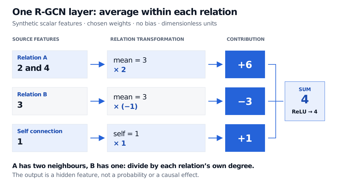
Here Nir contains the incoming neighbours under relation r, Wr transforms that relation's messages, and W0 transforms the node's own state. The original R-GCN paper, Eq. 2 permits different normalisers. We choose ci,r=∣Nir∣: average within each nonempty relation, then add the relation contributions. An empty relation contributes zero.
Use scalar, dimensionless features and stipulated weights, with no bias:
Channel
Incoming features
Weight
Contribution
Relation A
2 and 4
2
2(2+4)/2=6
Relation B
3
−1
(−1)3/1=−3
Self
1
1
1
With a ReLU activation,
hi′=max(0,1+6−3)=4.
Synthetic scalar R-GCN layer: relation A features 2 and 4 average to 3 and weight 2 gives 6; relation B feature 3 and weight minus 1 gives minus 3; self contributes 1. Their sum is 4 and ReLU outputs 4.
Original synthetic R-GCN calculation. Each relation uses its own neighbour count; all features and outputs are dimensionless and all weights are chosen by hand.
The negative weight changes the message's sign; it is not a negative probability or a learned attention weight. Without the degree normalisation, these same inputs would give 1+2(2+4)−3=10. Neither convention is automatically correct for every application. A mean reduces sensitivity to relation degree, but also loses count information unless that is supplied separately.
The output 4 is a hidden feature. A task-specific prediction head must turn representations into a forecast or classification. For knowledge-graph link scoring, an encoder can instead feed a separate triple-scoring decoder. Message passing and triple scoring are distinct components. DGL’s official R-GCN tutorial describes the different downstream heads.
Financial edges must be eligible at prediction time
Suppose a fictional supply relationship takes effect on 1 March but becomes usable by the research system on 8 March. A prediction made at noon UTC on 5 March cannot use that edge just because its effective date is earlier. Keep effective intervals and disclosure/usable timestamps separately. The same restriction applies to node features: an eligible company node does not make its later revised accounts eligible.
Build the neighbourhood from the information available at the prediction cutoff. Apply that rule before computing relation degrees, sampling neighbours or producing embeddings: a future edge can alter a normaliser even if its message is later removed. At each training cutoff, use only eligible labels and fit preprocessing on the permitted training data. A chronological split of the final prediction table does not repair embeddings computed from a future graph. This applies the general data-leakage principle to graph construction.
The Observation, Event and Availability Timestamps lesson develops the clock distinctions and feasible decision ordering (public preview; full lesson requires membership). A temporal graph network addresses evolving graph state; simply attaching dates to a static R-GCN does not define an event-update policy.
Finally, a typed edge is an asserted relationship, not an identified causal mechanism. A useful distress prediction does not establish causal contagion along supplier links. Compare against simpler own-feature and neighbour-summary baselines under the same information cutoffs. Rare relation types also have few observations from which to estimate separate transformations; the original R-GCN's basis sharing and block structure are ways to constrain those parameters, rather than reasons to assume every relation has been learned reliably. Schlichtkrull et al., §2.2.