Reinforcement learning from human feedback: Definition & Examples

Reinforcement learning from human feedback (RLHF) trains a decision policy using human judgments as feedback, commonly by learning a reward model from comparisons and then optimizing that reward with reinforcement learning. For a quant research assistant, it can encourage summaries that analysts prefer. Preference for a summary does not establish that its financial claims are correct or that a strategy based on it will make money.

RLHF extends beyond language models. Christiano et al., §§2.1–2.2, learned rewards from human comparisons of short behavior clips and used them to train agents. A large language model provides a useful text example: the policy generates a response, and human feedback helps specify which responses are desirable.

One common pipeline

A widely used formulation has three stages, described in Ouyang et al., §§3.1 and 3.5:

Supervised fine-tuning (SFT). Train a pretrained model on demonstrations of desired responses.
Preference and reward learning. Have people compare responses to the same prompt. Fit a scalar reward model to those comparisons.
Policy optimization. Generate responses and update the policy using the learned reward, with a penalty for departing from a reference policy.

These are different learning tasks. Demonstrations supply responses to imitate; comparisons supply choices to predict; reinforcement learning changes what the policy generates. This describes one pipeline, rather than a requirement that every post-training method use identical stages.

What does a reward of 2 mean?

Let $x$ be a prompt and $y_A,y_B$ two responses. A Bradley–Terry preference model assigns

P(y_A\succ y_B\mid x) =\sigma\big(r_\phi(x,y_A)-r_\phi(x,y_B)\big), \qquad \sigma(z)=\frac{1}{1+e^{-z}}.

The event is “a labeler prefers A to B.” The scalar

r_\phi

is learned to predict such choices. This formulation assumes a common scalar preference score at a fixed logistic scale; conflicting or context-dependent judgments need not fit it well. Christiano et al., §2.2.3, explain the preference-prediction interpretation and the comparison loss.

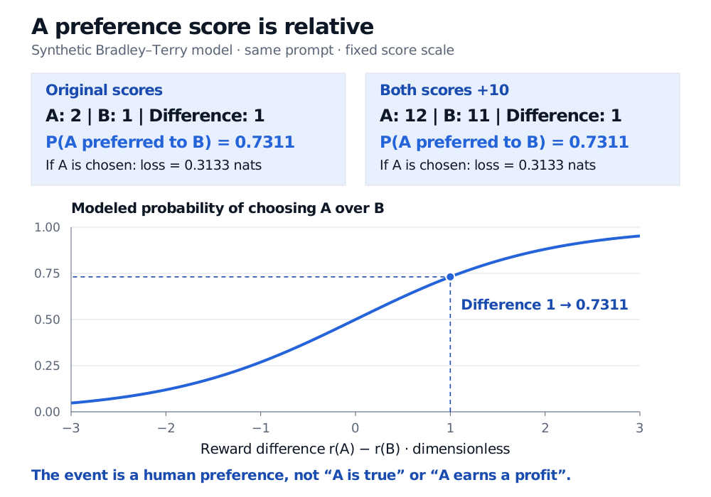
Consider a synthetic comparison of two summaries of the same filing. Suppose the reward scores are

r_A=2

and

r_B=1

. Then

P(A\succ B)=\sigma(1)\approx0.7310585786.

If the human chooses A, that observation contributes negative log-likelihood

\ell=-\ln P(A\succ B)\approx0.3132616875\text{ nats}.

Training minimizes the average loss over preferred/dispreferred pairs. A higher probability for the observed choice gives a lower loss. It does not certify the content of that choice.

Synthetic Bradley–Terry scores A=2 and B=1 imply a preference probability of 0.7311 and chosen-A loss of 0.3133 nats. Scores A=12 and B=11 give identical results because both have difference 1. The logistic curve maps reward difference to preference probability.

Original synthetic comparison at a fixed logistic scale. Only the score difference determines this pairwise probability; the scores have no currency or return units.

Adding 10 to both scores gives $12-11=1$ , so both the probability and the loss remain unchanged. Absolute reward levels are therefore not identified by these pairwise comparisons. Multiplying both scores by a constant generally changes the predicted probability: shift invariance is not scale invariance.

The number 0.7311 is neither a 73.1% probability that A is true nor a predicted probability of a profitable trade. Even its interpretation as a preference probability needs testing on held-out judgments. Probability calibration must name the event being calibrated.

Turning the score into a policy objective

Write $\pi_\theta(y\mid x)$ for the probability of a complete response, $\pi_{\mathrm{ref}}$ for a fixed reference policy, and $D$ for the training prompt distribution. A common regularized objective is

\max_\theta\;\mathbb{E}_{x\sim D}\left[ \mathbb{E}_{y\sim\pi_\theta(\cdot\mid x)}[r_\phi(x,y)] -\beta D_{\mathrm{KL}}\!\left( \pi_\theta(\cdot\mid x)\,\Vert\,\pi_{\mathrm{ref}}(\cdot\mid x) \right)\right],\qquad\beta>0.

Here the reward model is held fixed during the policy optimization stage; the reference is often the SFT policy. The KL term penalizes distributional departure, with larger

\beta

penalizing it more strongly at a fixed reward scale. Finite KL requires reference support wherever the new policy assigns probability. Rafailov et al., §3, give this objective.

Ouyang et al. used proximal policy optimization (PPO) for the policy updates. The reference-policy KL penalty belongs to the training objective; it is distinct from PPO's control of individual policy updates. A penalty can restrain optimization of an imperfect reward model, but it is no guarantee of factual accuracy or compliance with a hard constraint.

Where DPO differs

Direct preference optimization (DPO) fits the policy directly to preference pairs, without a separately trained reward network or a PPO training loop. In the original Bradley–Terry derivation, its pair loss is

\ell_{\mathrm{DPO}}=-\ln\sigma\!\left( \beta\ln\frac{\pi_\theta(y_w\mid x)}{\pi_{\mathrm{ref}}(y_w\mid x)} -\beta\ln\frac{\pi_\theta(y_l\mid x)}{\pi_{\mathrm{ref}}(y_l\mid x)} \right),

where

y_w

is preferred and

y_l

dispreferred. Rafailov et al., §4, derive this from the regularized reward objective through an implicit reward parameterization. That connection depends on the preference model and reference-policy setup; it does not make arbitrary preference training equivalent to PPO-based RLHF.

A financial summary still needs evidence

Suppose reviewers favor a concise earnings summary that confidently calls a one-off gain “recurring profit.” A preference-trained model can learn the presentation reviewers reward while preserving that accounting error. The score is only as useful as the judgments, instructions and examples behind it. Ouyang et al., §§5.2–5.3, explicitly discuss whose preferences their labels represent and continuing factual mistakes.

For this research use, evaluate separate questions: Does each claim match the filing, entity, period and units? Do held-out analysts prefer the summary under an explicit rubric? Does any resulting investment rule work on subsequently available data after costs? A higher reward answers none of those questions by itself. Approval requirements and trading limits must be enforced separately from a learned preference score.

The Measurement Validity lesson develops the distinction between agreement with a label and measuring the intended financial construct. The LLM Annotation lesson explains fixed codebooks and audited human–model comparisons. Both offer public previews; full lessons require membership.

Sources

Paul F. Christiano et al., Deep Reinforcement Learning from Human Preferences, 2017, §§2.1–2.2.3: behavior comparisons, reward fitting and policy training. The cited version also describes modifications beyond the basic preference model used in the synthetic example.
Long Ouyang et al., Training Language Models to Follow Instructions with Human Feedback, 2022, §§3.1, 3.5–3.6 and 5.2–5.3: SFT, reward modeling, PPO, reference regularization and feedback limitations. This is a historical training study, not a statement about any current vendor product.
Rafael Rafailov et al., Direct Preference Optimization: Your Language Model is Secretly a Reward Model, 2023; cited revision 2024, §§3–4: preference likelihood, KL-regularized objective and direct preference loss.

One common pipeline

What does a reward of 2 mean?

Turning the score into a policy objective

Where DPO differs

A financial summary still needs evidence

Sources

Related terms

Large language model

Reinforcement learning