Test for a unit root with one externally fixed break date. Distinguish break dummies, model-specific nulls and critical values from endogenous-date testing.
Perron known-break unit-root test
A Perron known-break unit-root test tests for a unit root while allowing one structural break at a date fixed outside the test's search procedure. Its practical purpose is to distinguish persistent stochastic shocks from fluctuations around a broken deterministic trend. Otherwise, a regime shift in a macroeconomic input can look like evidence that every shock has a permanent effect.
“Known” is a statistical assumption about date selection. Naming a historical event after inspecting the series does not automatically justify treating its date as exogenous. Perron's original study treated the 1929 crash and 1973 oil shock dates as fixed. Perron (1989), §§1–2
A break has different meanings under the two hypotheses
Let TB be the last pre-break period. Define a step, a centred trend change and a one-period pulse:
DUt=1{t>TB},DTt∗=(t−TB)DUt,Pt=1{t=TB+1}.
The original three cases distinguish a level shift, a slope change, and both. With et a stationary short-memory disturbance, their basic hypotheses can be written as follows; parameters are specific to each row.
Case
Unit-root null
Broken-trend stationary alternative
A: crash
yt=yt−1+μ+dPt+et
yt=a+bt+cDUt+et
B: changing growth
yt=yt−1+μ+gDUt+et
yt=a+bt+hDTt∗+et
C: both
yt=yt−1+μ+dPt+gDUt+et
yt=a+bt+cDUt+hDTt∗+et
A pulse in the null's change equation can permanently shift the level because the unit root carries it forward. A step changes the drift. Under the alternative, ordinary disturbances dissipate around the specified broken trend. The whole level series need not be covariance-stationary. The centred representation of C spans the same deterministic terms as Perron's original uncentred tDUt, but its level-shift coefficient has a different interpretation. Perron (1989), §2
Eight periods: understand the dummies before testing
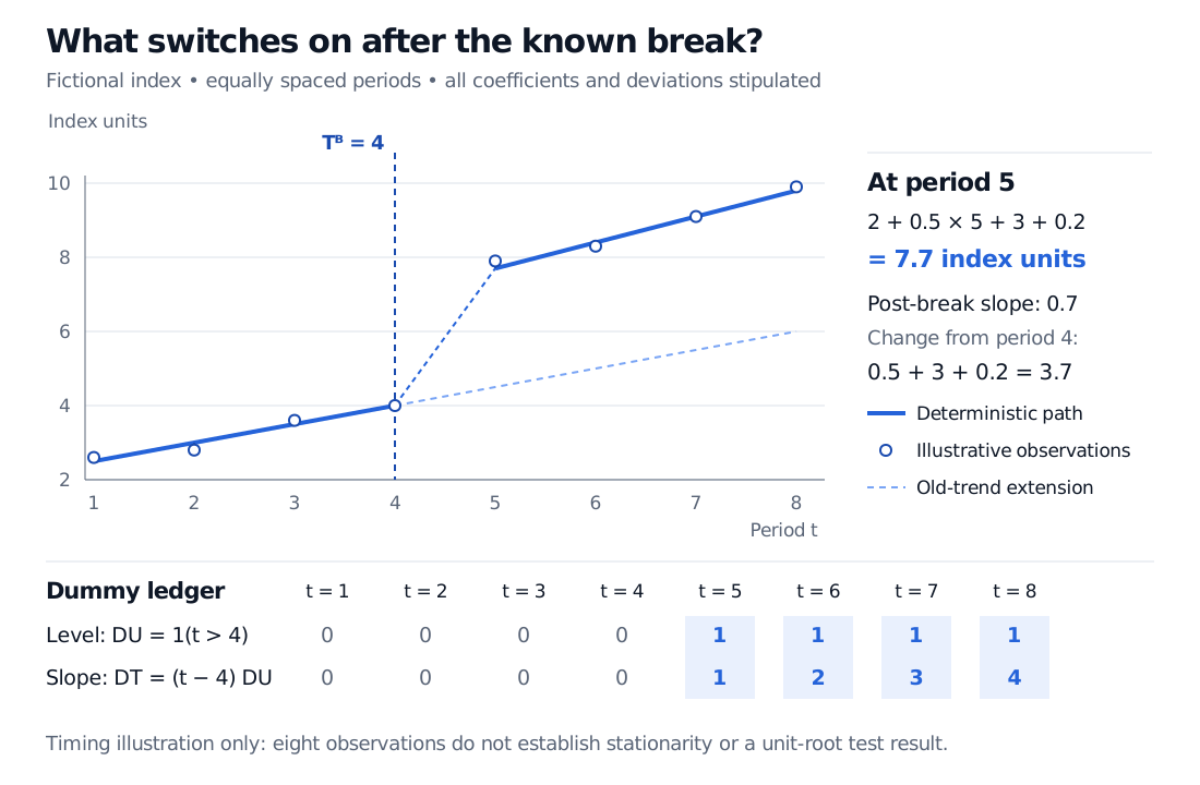
Take a fictional index with TB=4 and the stipulated component
mt=2+0.5t+3DUt+0.2DTt∗.
Its values for periods 1–8 are 2.5,3,3.5,4,7.7,8.4,9.1,9.8. Adding the declared deviations 0.1,−0.2,0.1,0,0.2,−0.1,0,0.1 produces the observations in the figure.
Fictional eight-period index: deterministic path 2.5, 3, 3.5, 4, 7.7, 8.4, 9.1, 9.8; observations 2.6, 2.8, 3.6, 4, 7.9, 8.3, 9.1, 9.9. The known break follows period 4; DU switches to one at period 5 and the centred slope dummy takes values 1, 2, 3, 4 thereafter.
Fictional index with stipulated coefficients and deviations. The solid blue segments show the deterministic component; circles show observations and the pale dashed line extends the old trend. The ledger fixes the dummy timing. No model is fitted.
The post-break slope is 0.5+0.2=0.7 index units per period. The coefficient 3 is the level-shift parameter, while the first post-break change is 7.7−4=3.7: the old slope contributes 0.5, the level shift 3, and the new slope increment 0.2. Relative to the old-trend value at period 5, the gap is 3.2. Confusing these quantities changes the model being described.
These eight points demonstrate timing arithmetic. They provide neither a fitted test statistic nor a p-value, and cannot establish stationarity.
The regression and its reference distribution travel together
For the innovational-outlier version of C, an augmented regression is
The null imposes α=1 and β=γ=0; the step and pulse can remain. For the corresponding A regression, omit DTt∗; its null also imposes θ=0. The statistic is the t-ratio for α=1, interpreted in the left tail using the appropriate break-test distribution. The lag augmentation addresses serial dependence. Ordinary Student-t or unchanged ADF cutoffs do not follow merely from adding dummy variables. Reference values depend on the specification and break fraction λ=TB/T. Perron, Dealing with Structural Breaks, §5.3
The transition assumption also matters. An additive outlier changes the deterministic component immediately; an innovational outlier transmits the intervention through the process's dynamics. Additive-outlier procedures first remove the broken trend, then test the residual process with the required pulse controls. A slope-only model with joined trend segments needs its own procedure and reference distribution; it is not recovered by silently dropping a variable from the general regression. Perron's later review incorporates corrections to the original additive-outlier treatment. Perron, §§5.1–5.3
If the date was searched, change the test
The Zivot–Andrews test chooses a break date from candidate dates using the most negative unit-root statistic. Its reference distribution accounts for that search; fixed-date Perron critical values cannot be reused. Its original null is also a unit-root process without a break, against a broken-trend stationary alternative. It is therefore more than Perron's test with an estimated date substituted. Failure to reject either test is not proof of a unit root; weak power and specification errors remain possible. Zivot and Andrews (1992), §§1–2 and conclusion
For the regression-testing foundation, Testing for Unit Roots: Dickey–Fuller, ADF, and Phillips–Perron develops lag augmentation, deterministic terms and nonstandard critical values. The public page previews the lesson; the full teaching requires membership.