PAC-Bayes bound: Definition & Examples

A PAC-Bayes bound is a probabilistic generalisation guarantee for a learned distribution over predictors. It relates training loss to population loss through a penalty for moving that distribution away from a fixed prior. For a quant researcher, it makes the cost of adapting a randomised forecasting model to data explicit—under the theorem's sampling and loss assumptions.

“PAC” means probably approximately correct. Unlike a bound stated only through the size of a hypothesis class, PAC-Bayes can use the particular distribution learned from the data. Dziugaite and Roy (2017) demonstrate this approach for stochastic neural networks.

Which predictor receives the guarantee?

Let

P

be a prior distribution over candidate predictors and

Q

a learned distribution over the same space. A Gibbs predictor samples a predictor

h\sim Q

to make its prediction. Its risk averages loss over this random draw and a fresh observation. A deterministic classifier obtained from mean weights, averaged scores or majority voting is a different object; the same risk guarantee does not transfer automatically. Dziugaite and Roy, §§1–2, make the stochastic-model distinction explicit.

The word posterior here names

Q

. It need not be obtained by Bayesian inference. Any data-dependent learning procedure may choose it. By contrast, a Bayesian posterior follows likelihood times prior, normalised; Bayesian Reasoning develops that updating rule (full lesson requires membership; public preview available).

One exact PAC-Bayes-kl statement

Use the finite data and predictor spaces of Maurer's Theorem 5. Fix a loss

\ell(h,z)\in[0,1]

, a prior

P

independent of the sample, and

\delta\in(0,1)

. Draw

S=(z_1,\ldots,z_n)

independently and identically from

D

, with

n\ge8

. Define

\widehat L_S(Q)=\mathbb{E}_{h\sim Q}\left[\frac1n\sum_{i=1}^n\ell(h,z_i)\right], \qquad L_D(Q)=\mathbb{E}_{h\sim Q}\mathbb{E}_{z\sim D}[\ell(h,z)].

With probability at least

1-\delta

over

S

, simultaneously for every distribution $Q$ ,

\operatorname{kl}\!\left(\widehat L_S(Q)\,\|\,L_D(Q)\right) \le \frac{\operatorname{KL}(Q\|P)+\ln(2\sqrt n/\delta)}{n}.

This simultaneous guarantee permits choosing $Q$ after seeing $S$ . The confidence concerns repeated training samples, rather than a posterior probability that an individual fitted model is correct. Finite spaces keep measurability simple; continuous-space versions require the corresponding measurable setup.

Two KL quantities, two jobs

The left side compares Bernoulli distributions whose means are risks:

\operatorname{kl}(a\|b) =a\ln\frac ab+(1-a)\ln\frac{1-a}{1-b}.

At zero and one, use the limiting conventions: a zero-mass term contributes zero; positive mass against a comparison event of probability zero gives infinite divergence.

The right side uses relative entropy between distributions over predictors. These are different arguments of the same divergence construction, not interchangeable inputs. The Bernoulli expression is valid for bounded risks even when individual losses are not binary. To upper-bound population risk, find the largest admissible value

b\in[0,1]

satisfying the kl inequality for the observed empirical risk. Dziugaite and Roy (2018), §4, distinguish these quantities and describe this inversion.

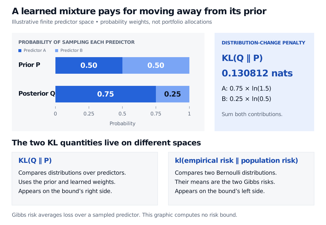
Consider two fictional predictors, A and B. Give each prior probability $0.5$ , then learn posterior probabilities $0.75$ and $0.25$ . Using natural logarithms,

\begin{aligned} \operatorname{KL}(Q\|P) &=\sum_{h\in\{A,B\}}Q(h)\ln\frac{Q(h)}{P(h)}\\ &=0.75\ln(1.5)+0.25\ln(0.5)\\ &\approx0.130812\text{ nats}. \end{aligned}

The B contribution is negative; only their sum must be nonnegative. These weights are probabilities of sampling predictors, not portfolio allocations. The result alone says nothing about the predictors' losses: sample size, confidence and empirical Gibbs risk are still needed for a numerical risk bound. Putting posterior mass where the prior assigns zero makes the KL penalty infinite.

Illustrative two-predictor example: prior weights are 0.5 and 0.5; posterior weights are 0.75 and 0.25. KL(Q relative to P) is 0.130812 nats. This predictor-space penalty differs from Bernoulli kl comparing empirical and population Gibbs risks.

Original illustrative example. The bars show probabilities of sampling predictors A and B. The numerical calculation is the posterior-to-prior KL penalty only; no risk bound is calculated.

The prior cannot quietly follow the same sample

Setting

P=Q

after fitting would erase the penalty, but violates the fixed-prior theorem. Valid data-dependent-prior results exist: Dziugaite and Roy (2018), Theorem 4.2, use a differentially private prior-selection mechanism and add terms to the bound. Such a result needs its own conditions; it is not permission to substitute a fitted prior into the displayed formula.

For financial data, serial dependence, overlapping labels and changing regimes obstruct the i.i.d. premise. Unbounded return-based loss also falls outside this statement; bounding or clipping loss changes the target being certified. A small penalty alone neither establishes useful generalisation nor certifies future trading returns.

Sources

Maurer, A. (2004), A Note on the PAC Bayesian Theorem, §3, Theorem 5: finite-space bounded-loss theorem, simultaneous posterior guarantee and exact constants for $n\ge8$ .
Dziugaite, G. K. and Roy, D. M. (2017), Computing Nonvacuous Generalization Bounds for Deep (Stochastic) Neural Networks with Many More Parameters than Training Data, §§1–2: randomised predictors, their risks and PAC-Bayes learning.
Dziugaite, G. K. and Roy, D. M. (2018), Data-dependent PAC-Bayes priors via differential privacy, §4 and Theorem 4.2: risk-space kl, predictor-space KL and valid private data-dependent priors.

Which predictor receives the guarantee?

One exact PAC-Bayes-kl statement

Two KL quantities, two jobs

The prior cannot quietly follow the same sample

Sources

Related terms

Generalisation