Overconfidence can overstate ability, relative rank or certainty. Distinguish its three forms and assess a forecast without diagnosing psychology from one score.
Overconfidence bias
Overconfidence bias is excessive belief in one's ability, relative standing or the accuracy of one's knowledge. In quantitative research it can turn a noisy winning streak into an exaggerated estimate of skill, or an uncertain forecast into an unjustifiably concentrated position. The relevant question is what the researcher believes relative to the evidence and an appropriate benchmark.
“My strategy has more predictive skill than it actually has.”
Believed performance against a defensible estimate of performance.
Overplacement
“My forecasts beat those of comparable researchers.”
Relative rank against a clearly defined comparison group.
Overprecision
“The uncertainty around my estimate is very small.”
Whether the claimed certainty is justified; for forecast intervals, whether stated coverage matches outcomes.
These are distinct. A researcher can underestimate absolute performance while overestimating relative rank. Overprecision can concern an overly certain pessimistic belief as well as an optimistic one. Moore and Healy also show why task difficulty and the way confidence is elicited matter; “overconfidence” is not a single universal error rate.
After a hot streak: how success can distort learning
Several profitable trades are evidence to interpret. The distortion arises when success receives too much credit as proof of personal ability, while failures are attributed to circumstances without a comparable reassessment.
Gervais and Odean formalise this mechanism in Learning to Be Overconfident (2001), pp. 1–4. Their trader learns about signal quality but overweights successful signals when updating beliefs about ability. The resulting overconfidence is generated by the model's learning rule. It is a mechanism that can explain biased learning, not evidence that every successful trader is biased.
For a strategy researcher, a streak may also reflect market exposure, dependence between trades or selection among many attempted strategies. Backtest overfitting is a separate statistical selection problem: it can make a track record look unusually good even without anyone consciously exaggerating it. Crediting that selected record entirely to skill compounds the problem.
What an unjustified probability costs
Consider a fictional event: a signal correctly predicts the next return's direction. Stipulate that the true event probability is p=0.60, and that a forecaster always reports q=0.80. The true probability is known because we specified the toy data-generating process. It is not inferred from an observed trading record.
Let Y=1 for a correct prediction and Y=0 otherwise. Use the binary Brier score convention L(q,Y)=(q−Y)2, with lower loss better. Some categorical conventions sum both outcome components and give twice this value.
At q=0.80, the loss is 0.04 when the prediction is correct, but 0.64 when it is wrong. Averaging over the stipulated probabilities gives:
E[L(0.80,Y)]=0.60(0.80−1)2+0.40(0.80−0)2=0.28.
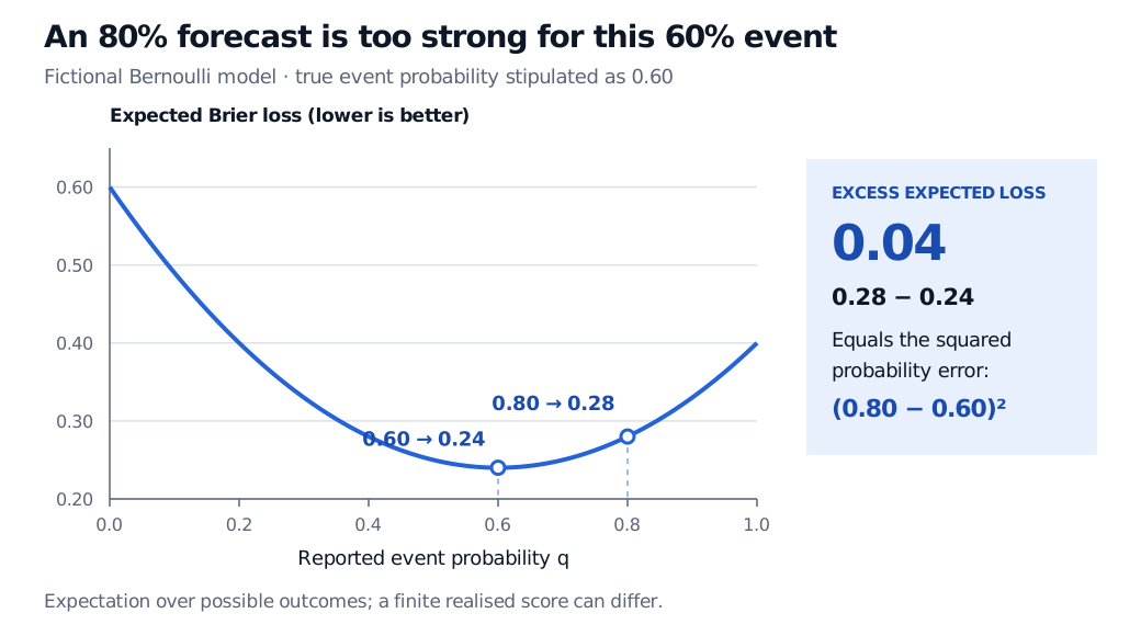
Reporting q=0.60 instead gives expected loss 0.24. Expanding the square isolates the cost of misreporting the probability:
E[(q−Y)2]=p(1−p)+(q−p)2.
Here, p(1−p)=0.24 remains even at the correct probability: the outcome is uncertain. The excess is (0.80−0.60)2=0.04. This calculation illustrates the strict propriety of Brier loss: its expected value is uniquely minimised at the true probability. See Gneiting and Raftery (2007), §1 and Table 1; their scores use the opposite sign, as rewards to maximise.
Fictional Bernoulli model: expected Brier loss is minimised at forecast 0.60 with loss 0.24; forecast 0.80 has loss 0.28, an excess of 0.04. The curve shows expectations, not a realised sample or a diagnosis.
Original stipulated-probability illustration. Greater reported certainty raises expected loss when it moves the forecast away from the true probability; no psychological cause is identified.
The expected number of correct predictions in 100 trials is 60. The observed count need not be 60, and even observing exactly 60 successes would not establish that the unknown probability is exactly 0.60. Likewise, one realised Brier score cannot identify overconfidence. Misspecification, changing conditions and incomplete information can also generate miscalibration.
Assess the forecast before judging the forecaster
A useful audit records the event definition, forecast horizon and probability before the outcome is known. Compare competing forecasts on the same resolved cases, preserve a genuinely out-of-sample evaluation, and inspect both proper scores and reliability: do comparable probability forecasts correspond to comparable event frequencies? Gneiting and Raftery's §2.3 explains why comparisons across different forecast situations can confound skill with task difficulty.
Finite samples leave uncertainty around these assessments. Sparse probability bins, overlapping return horizons and changing regimes make apparent calibration gaps harder to interpret. Assessing interval overprecision additionally requires matching the interval's stated target and coverage; uncertainty about a parameter and uncertainty about a future return are different objects.
High turnover is also insufficient as an individual diagnosis. Barber and Odean (2000), pp. 774 and 792–794, find that the highest-turnover households in their brokerage sample had much lower net returns than the lowest-turnover households, with much smaller gross-return differences. They interpret the evidence as consistent with overconfidence models. The study does not establish a universal performance penalty or identify every active investor's beliefs.
For the next step in forecast assessment, the Probability calibration lesson separates ranking from probability meaning and discusses held-out reliability checks. The public page is a preview; the full lesson requires membership.
Sources
Moore, D. A., and Healy, P. J. (2008). The Trouble With Overconfidence. Psychological Review, 115(2), 502–517. Definitions and measurement limitations, pp. 502–504.
Gervais, S., and Odean, T. (2001). Learning to Be Overconfident. Review of Financial Studies, 14(1), 1–27. Learning mechanism, pp. 1–4.
Barber, B. M., and Odean, T. (2000). Trading Is Hazardous to Your Wealth. Journal of Finance, 55(2), 773–806. Turnover comparisons and interpretation, pp. 774 and 792–794.