Nested clustered optimisation allocates within asset clusters, then across the resulting portfolios. Follow a four-asset example and see why clustering changes the feasible allocation.
Nested clustered optimisation
Nested clustered optimisation (NCO) is a portfolio allocation procedure that first optimises weights within groups of related assets, then optimises allocations across the resulting cluster portfolios. For a quant building a large portfolio, it replaces one joint allocation with smaller linked problems, aiming to contain the effect of unstable estimates among closely related assets.
The word nested describes those two allocation levels. It does not refer to nested cross-validation. Nor is NCO another name for hierarchical risk parity: HRP uses a tree and recursive risk-based allocation; NCO runs an allocation optimiser within clusters and again between them.
What is being nested?
López de Prado presents NCO as a wrapper around an allocation method, rather than one fixed objective. His original-author treatment clusters correlations; its example code uses repeated k-means fits, selects using silhouette quality and normalises portfolio weights to sum to one. The framework permits other clustering and allocation methods. Denoising the estimated covariance matrix is a separate preparation step, not a consequence of grouping assets. See the original treatment in Machine Learning for Asset Managers, §7.6.
For a fully invested minimum-variance implementation, let W contain one within-cluster portfolio per column, with zeros outside that cluster and each column summing to one. With asset covariance matrix Σ, the covariance of the cluster portfolios is
ΣC=W⊤ΣW.
Optimise cluster weights a using this reduced matrix, then recover asset weights:
w=Wa,1⊤a=1.
The budget follows automatically: 1⊤W=1⊤, so 1⊤w=1. Importantly, ΣC includes the covariance between the actual weighted cluster portfolios. Replacing it with a diagonal matrix just because the assets have been clustered discards information.
If expected returns enter the outer objective, their corresponding vector is W⊤μ. The objective, return convention and constraints must remain consistent across the reduction.
Four assets, two stipulated clusters
Consider fictional assets A, B, C and D with these population covariances for one-year simple returns, expressed in decimal-return-squared units:
Stipulate clusters AB and CD. This is an allocation calculation with known inputs, not a claim that a clustering algorithm inferred two groups from four observations. No return forecasts, cash asset, trading costs or weight bounds are included; signed weights are permitted, although the solution happens to be positive.
At each level use the fully invested global minimum-variance portfolio:
GMV(S)=1⊤S−11S−11.
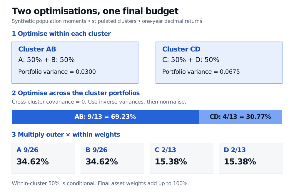
Within each pair, equal variances and symmetric covariance give weights of one half each. Thus
W=1/21/200001/21/2,ΣC=(0.03000.0675).
For example, the AB variance is (0.04+0.04+2×0.02)/4=0.03. The zeros between clusters come from this example's stipulated covariance, not from the NCO procedure.
Since the two cluster portfolios are uncorrelated, their minimum-variance weights are proportional to inverse variance:
aAB=1/0.03+1/0.06751/0.03=139,aCD=134.
Multiplying by the inner weights produces
w=(269,269,132,132)⊤.
A and B receive about 34.62% each; C and D receive about 15.38% each. The variance is 0.02076923. A 50% inner weight means half of that cluster's allocation, not half of total capital.
Synthetic NCO example: within each stipulated cluster AB and CD the weights are 50% each. Cluster variances are 0.0300 and 0.0675 with zero cross-covariance. Outer weights are 9/13 and 4/13; final asset weights are A and B 34.62% each, C and D 15.38% each.
Original synthetic one-year example. The inner weights describe each cluster portfolio; the outer weights allocate the total budget. Their products give the asset weights.
Why this is not a free improvement on optimisation
Directly solving the four-asset GMV problem gives the same weights here. Block independence and within-block symmetry make the inner solutions sufficient for the joint optimum. That equality is a special property of these inputs, not proof that NCO generally equals or outperforms a joint optimiser.
Once W is fixed, the outer problem can choose only portfolios of the form Wa. It cannot independently change the ratio of A to B. With general cross-cluster covariances, the best ratio within AB can depend on the holdings of C and D, so freezing it can exclude the joint optimum. Under the same known covariance and compatible budget constraints, a restricted minimum-variance problem cannot beat the unrestricted problem's in-sample minimum variance. The practical motivation is a possible improvement in estimated, out-of-sample allocations, where parameter error matters.
The original paper's abstract explicitly rejects the expectation that one optimisation method dominates in every setting. Useful evaluation therefore includes alternative cluster choices, estimation windows and realistic costs. A changing partition can generate turnover even when the outer weights look stable.
Constraints also need attention in asset space. For an asset cap wi≤ci, the reduced problem needs (Wa)i≤ci; merely applying the same numerical cap to each cluster does not enforce it. Long-only inner and outer weights are sufficient for long-only final holdings, but inner normalisation alone does not impose long-only investing. Singular inner or reduced matrices also require a suitable solver or regularisation; clustering does not guarantee invertibility.
For the allocation foundations, Mean-Variance Optimisation derives the budget-normalised solution used here and contrasts it with return-seeking objectives. The full lesson requires membership; a public preview is available.
Sources
Marcos López de Prado, Machine Learning for Asset Managers, Cambridge University Press, 2020, §§7.6–7.7; snippets 7.3–7.6. Supporting details: clustering snippet 4.1 and weight normalisation snippet 2.10.