Separate unexpected trade-direction information from liquidity compensation, and see why MRR coefficient recovery needs identified order-flow predictability.
Madhavan–Richardson–Roomans model
The Madhavan–Richardson–Roomans (MRR) model is a structural model of transaction prices that separates revisions in a security's expected value from the costs of supplying liquidity. Its central idea is that the informative part of a trade is its unexpected direction, after allowing for predictable order flow. A repeated buy and a surprise sell can therefore move prices by different amounts even when trade size is unchanged.
For a quant estimating spread decomposition, this matters immediately: the coefficient on today's trade sign combines information and liquidity costs. Reading that coefficient as a pure adverse-selection cost overstates what the regression identifies.
Madhavan, Richardson and Roomans published the model in The Review of Financial Studies in 1997. The detailed specification below follows their accessible November 1996 author manuscript, distinguished from the 1997 publication record.
Prices respond to the surprise in the trade
Let xt denote trade direction: +1 for buyer-initiated and −1 for seller-initiated transactions. Let μt be the market's expected asset value after seeing trade t, and let pt be its transaction price. The information update is
μt−μt−1=θ(xt−E[xt∣xt−1])+εt.
Here θ≥0 measures the value revision per unit of trade-direction surprise, and εt is a public-information innovation. Transaction prices also compensate liquidity providers:
pt=μt+ϕxt+ξt.
The parameter ϕ≥0 represents the cost of supplying liquidity. In the authors' interpretation it can cover processing costs, inventory costs, risk bearing and market-maker rents. The pricing disturbance ξt captures stochastic rounding from price discreteness or other transitory pricing effects. Neither ϕ nor this regression separately identifies each of those economic costs.
In the manuscript's Markov specification, E[xt∣xt−1]=ρxt−1, where ρ is the first-order autocorrelation of trade direction. Substituting the price equation at consecutive observations yields
Δpt=(θ+ϕ)xt−(ρθ+ϕ)xt−1+εt+ξt−ξt−1.
The current sign loads on both information and liquidity compensation. The lagged sign removes the previous transaction's liquidity component and the predictable portion of today's information update. The original manuscript's §§2.1–2.2 develops these equations and their identifying moment restrictions.
The zero indicator is an actual transaction
The manuscript also permits xt=0 for a transaction within the quoted spread, modelled as execution at the midquote. This is not a no-trade observation. Its probability is λ=P(xt=0). With unconditional buy/sell symmetry, E[xt]=0 and Var(xt)=1−λ.
Under the manuscript's symmetric Markov transition specification, define
γ=P(xt=+1∣xt−1=+1)=P(xt=−1∣xt−1=−1).
The probability of a midpoint transaction following either a buy or a sell is taken to be λ. After a buy, the probabilities of buy, midpoint and sell are therefore γ, λ and 1−γ−λ. Hence
E[xt∣xt−1=+1]=γ−(1−γ−λ)=2γ−(1−λ)=ρ.
Here γ conditions only on the previous sign; it does not also condition on the current transaction being nonzero. Thus γ and ρ are different objects. A midpoint transaction following a buy has surprise 0−ρ, rather than automatically having zero information content. Arbitrarily inserting zeros during periods with no trades would change the model and its estimation problem.
One buy history, two price changes
Consider a fictional reduced trade-time model containing only xt∈{−1,+1}. There are no zero-sign transactions, and public news and pricing noise are set to zero. Set
θ=0.02,ϕ=0.01,ρ=0.5,
with monetary coefficients in USD per share per unit of sign. Under a symmetric two-state Markov law, ρ=0.5 corresponds to a 75% chance of repeating the previous sign. Suppose the previous trade was a buy, xt−1=+1.
Current trade
Sign surprise xt−0.5
Efficient-value change
Transitory change ϕ(xt−xt−1)
Transaction-price change
Buy, xt=+1
+0.5
+0.01
0.00
+0.01
Sell, xt=−1
−1.5
−0.03
−0.02
−0.05
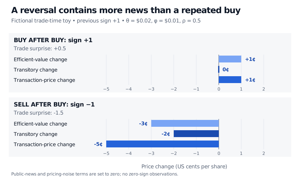
All price changes are USD per share. The repeated buy raises expected value by one cent; the transaction remains on the same side of value, so the liquidity component does not change. The reversal contains a larger negative information surprise and switches from the positive to the negative liquidity component. Its five-cent fall is therefore not all bid–ask bounce.
Fictional reduced MRR model after a buy: a repeated buy changes efficient value by plus one cent and the transitory component by zero; a sell changes them by minus three and minus two cents, giving a minus five-cent transaction-price move.
Original reduced-model example; price changes are US cents per share. Public news and pricing noise are zero, and only buy/sell observations are included.
What estimation must identify
Write the price regression as Δpt=b0xt+b1xt−1+ut. For the toy,
b0=0.03,b1=−0.02.
Once ρ is identified from trade-direction behaviour, the structural coefficients can be recovered, provided ρ=1:
θ=1−ρb0+b1,ϕ=b0−θ.
Here that gives θ=0.01/0.5=0.02 and ϕ=0.01. The two price-regression coefficients alone are insufficient: the same b0,b1 with ρ=0 instead imply θ=0.01 and ϕ=0.02. As ρ approaches one, division by 1−ρ makes the recovery sensitive to estimation error.
The authors use generalised method of moments to combine the price-regression restrictions with moments identifying trade-sign autocorrelation and the crossing probability. The differenced rounding disturbance ξt−ξt−1 also creates serial dependence even when rounding-error levels are independent; ordinary independent-error standard errors are inappropriate. A systematic tendency to round buys upward and sells downward can be absorbed into ϕ, further limiting a literal processing-cost interpretation.
Persistent buy signs do not prove informed trading. Order splitting, reporting conventions and other trading mechanisms can produce persistence; ρ describes that predictability. Interpreting θ as an information component relies on the model's value-update and orthogonality assumptions, rather than establishing a causal motive for each trade.
For empirical work, trade classification, quote timing and the treatment of inside-spread executions must match the specification. The owned Spread Measurement lesson connects those choices to effective and realised spreads and the restrictive Roll benchmark; its public preview is open and its full teaching requires membership. Those midpoint-based accounting measures complement MRR's structural estimates; they do not establish the same decomposition by definition.
The authors' November 1996 manuscript, FIN-96-034, especially §§2.1–2.2, printed pp.4–9, equations (1)–(3) and estimation moments; §3.1 on trade signing and quote timing. This is the accessible primary source for the detailed model discussed here.