Distinguish logistic Newton corrections, probability-based Real AdaBoost and SAMME class votes, with explicit score conventions and a three-class worked example.
LogitBoost, Real AdaBoost and multiclass AdaBoost
LogitBoost fits an additive classifier through weighted regression steps aimed at logistic loss. Real AdaBoost adds real-valued contributions derived from a weak learner's weighted class probabilities, using exponential loss. Multiclass AdaBoost names a family of extensions; SAMME is the discrete version that combines class predictions with an adjustment for the number of classes. These are distinct algorithms. For a quant classifying future price moves, credit events or execution outcomes, choosing between them changes the fitted correction, the sample weights and the meaning of the output score.
They share boosting's sequential structure: each new learner depends on the ensemble so far. They do not share one universal update rule.
Method
What the next learner supplies
Training criterion or mechanism
Binary LogitBoost
A regression function fitted to working responses
Newton-style steps for Bernoulli logistic loss
Binary Real AdaBoost
Weighted class-probability estimates
Half-log-odds contributions under exponential loss
Discrete SAMME
One of several class labels
A weighted vote under multiclass exponential loss
LogitBoost: state the score before the step
Use binary labels yi∈{0,1} and the full log-odds score G(x):
p(x)=1+e−G(x)1,L(y,G)=log(1+eG)−yG.
This is logistic regression's probability link, with an additive function rather than necessarily a single linear score. The loss gradient is p−y and its curvature is p(1−p). At each stage calculate
zi=pi(1−pi)yi−pi,wi=pi(1−pi).
Fit a regression learner h to zi using weights wi, then update G←G+h. The working response zi is a desired score correction, not a probability. A constrained learner, such as a shallow decision tree, usually approximates those corrections across many rows.
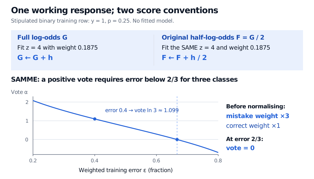
A stipulated training row. Let y=1 and the current p=0.25. Then w=0.25(0.75)=0.1875 and z=0.75/0.1875=4. The ordinary residual is 0.75; the Newton correction is 4 because it divides by curvature. This calculation does not imply that a fitted learner outputs exactly 4 at that row.
The original convention has a half. Friedman, Hastie and Tibshirani's Algorithm 3 uses F=G/2, so p=1/(1+e−2F). It fits the same working response z with the same weights, then applies F←F+h/2. Alternatively, a direct Newton correction expressed in F units is z/2, with curvature 4p(1−p). The factor belongs either in the correction or in the update, consistently. A common curvature multiplier does not change an unpenalised weighted least-squares minimiser; absolute penalty conventions require care.
For the stipulated row, an exact correction would add 4 to G, or 2 to F. Both give the same new probability. Dropping the half while retaining the original probability link doubles the intended full-score step. Optional shrinkage multiplies the consistent update by a learning rate; it does not repair a mixed convention.
When p is near zero or one, working responses can be extreme and curvature weights tiny. The original paper discusses response caps and weight floors. Such numerical protections, learner restrictions and shrinkage affect the fitted path; the display above is the unmodified arithmetic.
Real AdaBoost: probabilities from the reweighted sample
For Real AdaBoost, recode labels as y~i∈{−1,+1}. A learner fitted with the current observation weights returns qm(x), its estimate of the positive-class probability under that weighting. The stage contribution and reweighting are
followed by normalisation. Sum the contributions and classify by their sign. This is the exponential-loss construction in Algorithm 2 and Result 2, rather than LogitBoost's regression on Newton working responses.
For a separate stipulated leaf with weighted positive probability q=0.75, the contribution is 21log3≈0.5493. Its value varies with the input; discrete AdaBoost instead gives a stage's hard class prediction a common vote magnitude. Neither qm nor the final transformed score is automatically a calibrated probability for the original population. Probabilities of exactly zero or one also make the log ratio unbounded.
SAMME: why the extra class term matters
Let there be K mutually exclusive classes. Fit a weighted classifier Tm, and let ϵm be its weighted misclassification fraction. In the original, unshrunk discrete SAMME convention,
αm=logϵm1−ϵm+log(K−1).
Multiply mistaken rows' weights by eαm, leave correct rows' weights unchanged, then renormalise. Predict the class with the largest accumulated vote ∑mαm1{Tm(x)=k}. Zhu and coauthors' Algorithm 2 derives the extra term from multiclass exponential loss.
Three-class example. For K=3 and ϵ=0.4, α=log(1.5)+log2=log3≈1.0986. Before normalisation a mistake gets three times its old weight; a correct row gets once its old weight. The mistake group's total weight rises from 0.4 to 1.2/(1.2+0.6)=2/3. These are training weights, not predicted class probabilities.
The positive-vote condition is ϵ<1−1/K, so the three-class threshold is 2/3. It refers to the current weighted sample and the uniform-guessing benchmark, not a guarantee of useful financial prediction. At the threshold the vote is zero. Zero error makes the formula divergent and is handled as a stopping case in implementations. For two classes the extra term vanishes; this vote convention is twice the familiar half-log-ratio coefficient used with a signed binary exponential-loss score.
Stipulated binary row y equals 1 and p equals 0.25 gives working response 4 and curvature weight 0.1875. Full log-odds adds h; original half-log-odds adds h divided by 2. Three-class SAMME has vote ln 3, about 1.099, at weighted error 0.4; the vote reaches zero at error 2/3.
Original arithmetic and curve, with no model fitted. The two LogitBoost conventions give the same probabilities when their update scales are kept consistent. SAMME uses a different loss and a weighted class vote.
Multiclass does not mean one algorithm
Multiclass LogitBoost fits coupled class scores using a multinomial probability model, class-specific working responses and centred updates. It is not SAMME, nor merely several independent binary LogitBoost fits. The original paper's Algorithm 6 uses a quasi-Newton approximation; the softmax probabilities couple the classes.
SAMME.R is a probability-based real boosting extension. Its class log-probability contributions differ from SAMME's hard-label votes and error-based coefficient. Software names need a version: scikit-learn 1.5 exposed both options and deprecated SAMME.R; the current API, checked 1 November 2026, has no algorithm selector. The 1.6 documentation already states that only SAMME is implemented. An older example selecting SAMME.R therefore does not describe the current estimator.
For financial work, define classes and label horizons before training, preserve the availability of features and outcomes in validation, and examine class-specific errors and calibration. A loss-minimising classification score does not by itself specify a profitable position or account for transaction costs. Reweighting hard cases can also give mislabelled observations substantial influence.
Boosting: AdaBoost and Gradient Boosting develops the binary exponential-loss derivation and compares it with residual fitting. The full lesson requires membership; its public preview introduces the scope.