Least angle regression: Definition & Examples

Least angle regression (LARS) builds a linear-regression coefficient path by moving toward the predictors most associated with the current residual, sharing the direction when another predictor catches up. For a quant comparing many candidate forecasting inputs, this supplies a sequence of models to evaluate rather than committing immediately to a full least-squares fit.

It is a path-building algorithm, not an automatic choice of the best model. Its early fits can support feature selection, but entry order does not establish economic importance or causality.

The catch-up rule

Write the residual as

r=y-X\beta

and define

c_j=x_j^\top r

. Here “correlation” means this inner product, not a reported Pearson correlation coefficient. Center the response and predictors, and give each predictor unit Euclidean length. Handle the intercept separately through centering.

Starting from zero coefficients, LARS follows the predictor with largest

\lvert c_j\rvert

until another ties it. It then follows a direction equiangular to the active predictors, oriented by their residual-correlation signs. This preserves their equal absolute residual correlations until the next entry. Equal angles concern vectors in observation space; they do not generally mean equal coefficient increments. The original construction is in Efron and coauthors, §2.

Two predictors, one change of direction

Use four fictional observations with centered columns

\begin{aligned} x_1&=(0.5,\ 0.5,\ -0.5,\ -0.5)^\top,\\ x_2&=(0.5,\ -0.5,\ 0.5,\ -0.5)^\top,\\ y&=(2,\ 1,\ -1,\ -2)^\top=3x_1+x_2. \end{aligned}

Both columns have length 1 and $x_1^\top x_2=0$ . The response units are arbitrary; these are not estimated financial exposures.

At the origin, the inner products are $c_1=3$ and $c_2=1$ , so the first coefficient moves while the second stays zero. Along that segment,

r=(3-\beta_1)x_1+x_2,\qquad c_1=3-\beta_1,\qquad c_2=1.

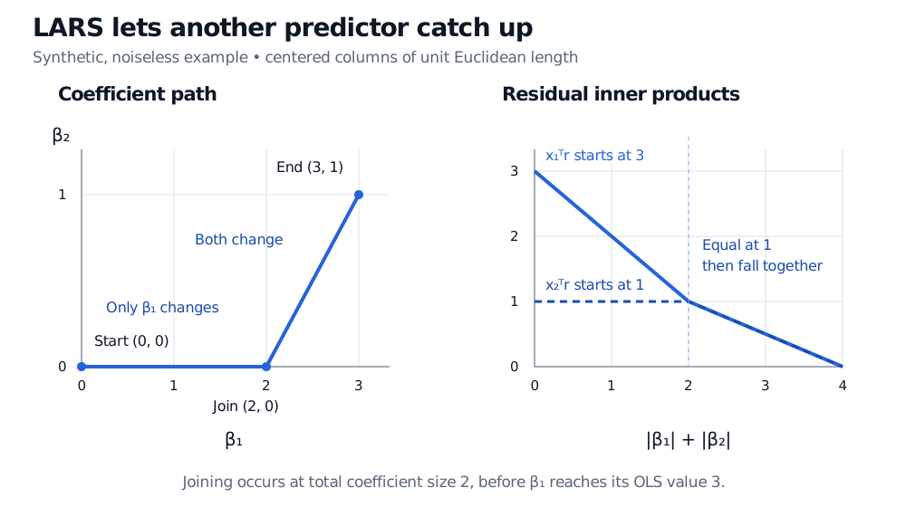
The second predictor catches up at

\beta_1=2

. The residual is then

(1,0,0,-1)^\top

, whose inner product with each column is 1. LARS changes direction here, before the first coefficient reaches its one-predictor least-squares value of 3.

With these orthogonal columns, the joint segment has coefficients $(\beta_1,\beta_2)=(2+a,a)$ for $0\le a\le1$ . Both residual inner products equal $1-a$ . The endpoint is $(3,1)$ , giving zero residual because this deliberately noiseless response lies in the span of the two columns.

Synthetic orthonormal example: the LARS coefficient path goes from (0, 0) to (2, 0) to (3, 1). Residual inner products start at 3 and 1, meet at 1 when the total coefficient size is 2, and then fall together to zero.

Original noiseless illustration. The horizontal axis on the right is total absolute coefficient size, not time or iteration count. Equal coefficient increments after entry are specific to this orthonormal design.

Zero training error is a property of this constructed example, not evidence that following a real forecasting path to its endpoint improves prediction.

The Lasso solves a penalized estimation problem. A modified LARS algorithm traces its path: stop a segment when an active coefficient reaches zero before the next entry, remove that predictor from the active direction, and continue. This prevents a nonzero Lasso coefficient from disagreeing in sign with its residual correlation. Unmodified LARS does not enforce that restriction. See the original paper, §3.1.

The paths coincide in this toy. Under the explicitly chosen objective

\frac12\lVert y-X\beta\rVert_2^2+\lambda\lVert\beta\rVert_1,

orthonormality gives $\beta_1=\max(3-\lambda,0)$ and $\beta_2=\max(1-\lambda,0)$ for $\lambda\ge0$ . Decreasing the penalty passes through the same knots. This special case does not establish equivalence for correlated designs.

Software conventions matter. The current scikit-learn path interface distinguishes the ordinary LARS path from the Lasso path. Its Lasso loss divides squared error by

2n

; this example uses a factor of

1/2

, so the same numerical penalty value has a different meaning. Unit-length scaling also differs from unit-variance scaling. Record preprocessing and objective normalization before comparing paths or penalties.

To choose a predictive fit, assess path positions on eligible held-out data, with centering, scaling and selection fitted inside each training window. For financial forecasts, respect chronology and label availability. Near-redundant predictors can make selected names unstable; a path is not a certificate of robust signal discovery. The SelfMadeQuant lesson Ridge, Lasso, and Elastic Net develops the penalty geometry; its public preview is open and the full lesson requires membership.

Finally, LARS also names an unrelated neural-network optimizer, Layer-wise Adaptive Rate Scaling, introduced by You, Gitman and Ginsburg. That method adapts learning rates by layer; it does not construct this regression path.

Sources

Efron, B., Hastie, T., Johnstone, I. and Tibshirani, R. (2004), Least Angle Regression, Annals of Statistics, 32(2), 407–451. §1, equation (1.1), §2 and §3.1: scaling, equiangular construction and Lasso modification.
scikit-learn developers, Linear Models, §§1.1.7–1.1.8, and lars_path reference. Current interface and objective conventions.
You, Y., Gitman, I. and Ginsburg, B. (2017), Large Batch Training of Convolutional Networks, abstract. Disambiguates the optimizer acronym.

The catch-up rule

Two predictors, one change of direction

LARS and Lasso are related, not interchangeable

Sources

Related terms

Feature selection

LARS and LAMB optimisers