K-means++ initialisation: Definition & Examples

K-means++ initialisation is a randomised way to choose starting centres for k-means, favouring observations far from centres already chosen. For a quant building asset peer groups, it addresses one source of variation in the fit: the starting locations. It does not decide which features make assets economically comparable.

The distinction matters because k-means clustering alternates nearest-centre assignments and mean updates. Those local improvements depend on where the centres start. K-means++ changes the starting rule; the subsequent Lloyd iterations still use the usual assignments and means.

Choose the next centre by squared distance

For an unweighted dataset of $n$ observations $x_i$ and a chosen cluster count $k$ , the original procedure is:

Select the first centre uniformly from the observations: each row has probability $1/n$ .
For every observation, calculate its distance to the nearest centre already selected:

D_i=\min_{c\in C}\lVert x_i-c\rVert.

Sample the next centre from the observations with probability

\mathbb{P}(\text{next centre}=x_i\mid C) =\frac{D_i^2}{\sum_{r=1}^{n}D_r^2}.

Recalculate these distances after each selection, until there are $k$ centres. Then run Lloyd's algorithm.

This is $D^2$ sampling, as defined by Arthur and Vassilvitskii, §2.2. It is neither deterministic farthest-point selection nor sampling proportional to unsquared distance. Already represented locations have zero weight. If the denominator is zero, every observed location is already covered and the seeding objective is zero; further selections require an explicit implementation convention rather than division by zero.

Three points expose the difference

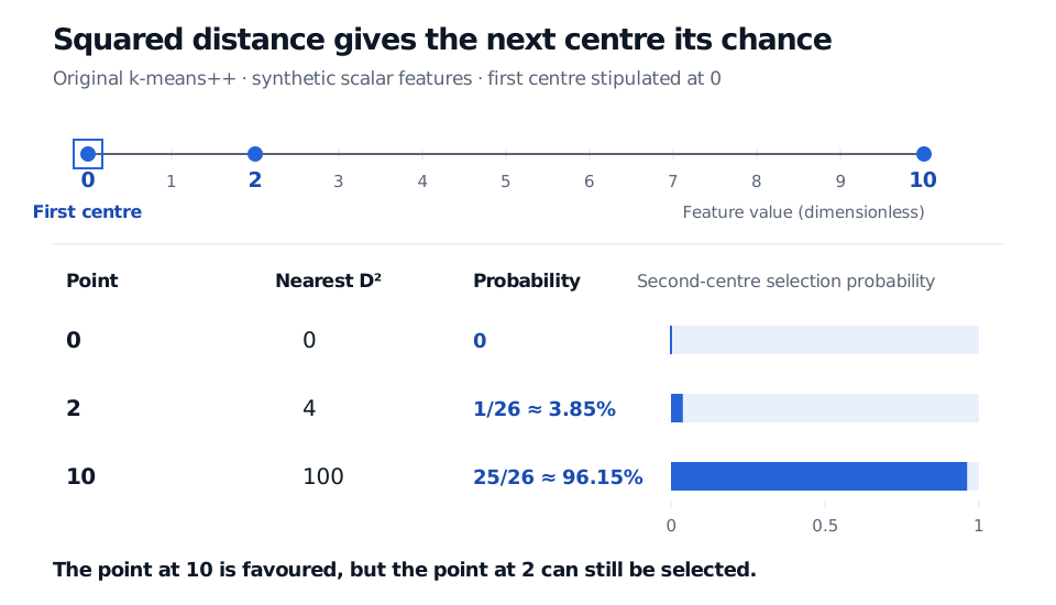
Take synthetic dimensionless scalar features

0,2,10

, with

k=2

. Condition on the first selected centre being

0

; we are stipulating this outcome, not replacing the uniform first draw.

Observation	Nearest-centre distance	Squared distance	Probability of being second
$0$	$0$	$0$	$0$
$2$	$2$	$4$	$4/104=1/26$
$10$	$10$	$100$	$100/104=25/26$

The observation at

10

is selected with probability about 96.15%, while the one at

2

retains about 3.85%. Unsquared-distance sampling would instead give the point at

2

probability

2/12=1/6

. Choosing the farthest point would give it zero probability. These are three different rules.

Synthetic dimensionless points 0, 2 and 10, with the first centre stipulated at 0. Squared nearest-centre distances are 0, 4 and 100; second-centre probabilities are 0, 1/26 (3.85%) and 25/26 (96.15%).

Original conditional seeding example. Bar lengths show probabilities, rather than distances; the distant point is likely but not certain to become the next centre.

Suppose the second centre is $10$ . The starting centres are then $0$ and $10$ , and the nearest-centre squared-distance sum is $4$ : only the observation at $2$ contributes. One Lloyd mean update moves the first centre to $1$ , the mean of $0$ and $2$ , while the other stays at $10$ . The cost becomes

(0-1)^2+(2-1)^2+(10-10)^2=2.

The groups then remain unchanged. This separates choosing seeds from fitting centres: seeds are observations, but a fitted mean need not be one.

What the guarantee measures

Write $\Phi(C)=\sum_i\min_{c\in C}\lVert x_i-c\rVert^2$ and let $\Phi_{\mathrm{OPT}}$ be the smallest such cost over all sets of $k$ centres. The original bound is

\mathbb{E}[\Phi(C_{\mathrm{seed}})] \leq 8(\ln k+2)\Phi_{\mathrm{OPT}}.

It holds in expectation over the random seeding, already before Lloyd iterations. Exact assignment and mean-update steps cannot increase that objective. The bound concerns a squared-distance cost, not the probability of recovering a “true” partition, and does not certify a global optimum for an individual run. See Theorem 3.1.

For financial features, the distance geometry still needs scrutiny. Multiplying one coordinate by $a$ multiplies its squared-distance contribution by $a^2$ , affecting both the next-seed probabilities and the fitted groups. A large isolated observation may attract a seed because its squared error is large; that alone does not make it an economically useful regime or peer group. Inspect feature scaling and unusual observations before attaching a financial interpretation.

Check the implementation's meaning of “++”

Scikit-learn's KMeans(init='k-means++') uses a greedy variant: it tries several candidates at a selection step and keeps the best. The probabilities above describe the original single-candidate rule. Its current n_init='auto' setting uses one run for this initialisation; using “++” therefore does not imply multiple restarts. Set the restart count explicitly when comparing fits, and record the random seed for reproducibility. These behaviours are documented under KMeans parameters.

For the assignment and mean-update mechanism after seeding, the SelfMadeQuant k-Means Clustering lesson develops the objective and alternating minimisation (membership; public preview).

Sources

David Arthur and Sergei Vassilvitskii, k-means++: The Advantages of Careful Seeding, §§2.1–2.2 and Theorem 3.1. Original paper, mirrored PDF.
Scikit-learn, KMeans: init, n_init and random_state. Current documentation checked 1 November 2026.

Choose the next centre by squared distance

Three points expose the difference

What the guarantee measures

Check the implementation's meaning of “++”

Sources

Related terms

Clustering