Natural gradient and Kronecker-factored approximate curvature: Definition & Examples

Natural gradient preconditions a probabilistic model’s loss gradient with its Fisher information matrix. Kronecker-factored approximate curvature (K-FAC) makes this idea tractable for neural networks by replacing large curvature blocks with products of smaller matrices. For a network estimating return distributions or derivative prices under a specified likelihood, this changes how training steps respond to differently scaled parameters. It does not establish that the fitted financial model generalises.

A step measured in predictions

Let $p_\theta(y\mid x)$ be a conditional predictive distribution, and let $L(\theta)$ be the average negative log-likelihood on the training data. Write its parameter gradient as $h=\nabla_\theta L$ . With score $s=\nabla_\theta\log p_\theta(y\mid x)$ , define

F=\mathbb{E}_{x\sim\hat q,\,y\sim p_\theta(\cdot\mid x)}[ss^\top].

Here

\hat q

is the empirical distribution of training inputs. The expectation over outputs still uses the model distribution. Where

F

is invertible, the natural gradient is

F^{-1}h

and a descent step has sign

-F^{-1}h

Locally, the average Kullback–Leibler divergence from the current predictions to the perturbed predictions is approximately

\tfrac12\delta^\top F\delta

. Minimising the linearised loss subject to a small budget on this quantity gives a direction proportional to

-F^{-1}h

. Thus a parameter change that strongly alters predictions is expensive even when its Euclidean length is small. This is a local statement; finite steps and damping require additional care. Martens (2020), Sections 5–6 and 10 develops that interpretation.

Using observed training labels in each score outer product instead produces the empirical Fisher, in the machine-learning terminology used here. This changes the curvature estimate, rather than merely making a Monte Carlo estimate of the same output expectation. Neither matrix is generally the training loss’s Hessian. Kunstner, Balles and Hennig, Sections 3–4 explain the distinction and its optimisation consequences.

Two approximations, not an independence theorem

For one dense layer, let $z=Wa$ , with $a\in\mathbb{R}^{n}$ and $W\in\mathbb{R}^{m\times n}$ . Biases are omitted here; they can be included by appending a constant input. For a model-sampled output, let $g$ be the derivative of its negative log-likelihood with respect to $z$ . The single-example weight derivative is $ga^\top$ .

With column-stacking vectorisation,

\operatorname{vec}(ga^\top)=a\otimes g

. The layer’s Fisher block and its K-FAC approximation are

\begin{aligned} F_{WW}&=\mathbb{E}[(aa^\top)\otimes(gg^\top)]\\ &\approx A\otimes G,\qquad A=\mathbb{E}[aa^\top],\quad G=\mathbb{E}[gg^\top]. \end{aligned}

The Kronecker product factorisation replaces an expectation of products with a product of expectations. It need not be exact: activations and backpropagated derivatives are generally dependent. The block-diagonal variant also discards cross-layer Fisher blocks. These are separate approximations. The original Martens–Grosse paper, Sections 2–3 also develops a variant with a block-tridiagonal approximate inverse; K-FAC is not defined solely by dropping all cross-layer terms.

Four weights, two solves

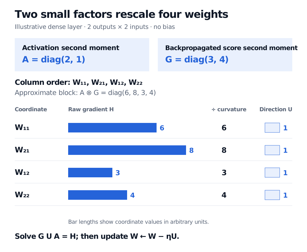
Consider a stipulated, illustrative layer with two outputs, two inputs and no bias. Choose second-moment factors and an average loss gradient $H=\nabla_W L$ as

A=\begin{pmatrix}2&0\\0&1\end{pmatrix},\qquad G=\begin{pmatrix}3&0\\0&4\end{pmatrix},\qquad H=\begin{pmatrix}6&3\\8&4\end{pmatrix}.

These factors specify an approximate block, not an assertion about an exact network Fisher. Stacking columns gives

\widetilde F=A\otimes G=\operatorname{diag}(6,8,3,4),\qquad \operatorname{vec}(H)=\begin{pmatrix}6\\8\\3\\4\end{pmatrix}.

Solving $\widetilde F u=\operatorname{vec}(H)$ yields $u=(1,1,1,1)^\top$ . Equivalently, keep the gradient in matrix form and solve

GUA=H,\qquad U=G^{-1}HA^{-1}=\begin{pmatrix}1&1\\1&1\end{pmatrix}.

A learning rate $\eta$ then gives $W_{\mathrm{new}}=W-\eta U$ . The four different raw gradient entries become equal direction entries because the chosen approximate curvature entries scale in the same proportions. This equality is a property of these illustrative numbers.

Illustrative two-output, two-input layer. A has diagonal 2 and 1; G has diagonal 3 and 4. In column order W11, W21, W12, W22, raw gradients 6, 8, 3, 4 divided by approximate curvature entries 6, 8, 3, 4 give direction entries 1, 1, 1, 1.

A deliberately diagonal example isolates the column-stacking convention. Real K-FAC factors can be dense and mix coordinates within a layer.

For an $m$ -output, $n$ -input layer, a full block has shape $mn\times mn$ ; the factors have shapes $n\times n$ and $m\times m$ . The identity $\operatorname{vec}(GUA)=(A^\top\otimes G)\operatorname{vec}(U)$ explains the two smaller solves. Since $A$ is symmetric, the ordering above follows. Changing the vectorisation convention without changing the Kronecker ordering gives the wrong operator.

Damping changes the solve

The inverse notation assumes nonsingular factors. With few samples or redundant activations, factors can be singular or poorly conditioned. Solving linear systems avoids explicitly forming inverses, but does not cure that sensitivity. The Numerical Conditioning and Stability lesson explains the issue; its preview is public and its full teaching requires membership.

Adding $\lambda I$ to the approximate block, with $\lambda>0$ , makes a positive-semidefinite block positive definite. It is generally different from adding a ridge to each factor:

(A+\alpha I)\otimes(G+\beta I) =A\otimes G+\beta A\otimes I+\alpha I\otimes G+\alpha\beta I.

The extra terms show why factor damping cannot silently stand in for $A\otimes G+\lambda I$ . A reported K-FAC step therefore needs its factor-estimation, cross-layer and damping conventions to be interpretable. Faster optimisation of a training likelihood remains a different question from out-of-sample forecasting performance.

Sources

Martens and Grosse (2015), Optimizing Neural Networks with Kronecker-factored Approximate Curvature, Sections 1–3: model Fisher, layer factorisation, structured inverse approximations and matrix-form updates.
Martens (2020), New Insights and Perspectives on the Natural Gradient Method, Sections 5–6, 8 and 10: natural-gradient geometry, the Hessian distinction and damping.
Kunstner, Balles and Hennig, Limitations of the Empirical Fisher Approximation for Natural Gradient Descent, Sections 3–4, version 3 (2020): model-output expectations versus observed-label outer products.