Seek representations with a common optimal predictor across training environments. Work through IRMv1’s gradient penalty and the limits of finite-environment invariance.
Invariant risk minimisation
Invariant risk minimisation (IRM) seeks a representation of the inputs on which the same predictor is optimal in every training environment. In quant research, the attraction is a return signal that survives changes in market conditions rather than exploiting one period’s accidental association. This is a learning objective, not a certificate of future stability. Arjovsky et al. (2019), §3
An environment is a labelled data source or condition with its own joint distribution of inputs and targets. For a financial application, a researcher might propose different venues or predetermined time blocks. Those choices are modelling hypotheses: two arbitrarily named subsets need not expose the relationships likely to break after deployment.
What has to be shared?
Let Φ be a representation, w its last-layer predictor and Re expected prediction loss in environment e. The ideal constraint is
Φ,wmine∈Etr∑Re(w∘Φ)subject tow∈argwˉminRe(wˉ∘Φ)for every e.
The last-layer function class matters. One pooled fitted model is insufficient: each environment must also prefer that same last layer, conditional on the representation. Equal prediction losses are not required. Arjovsky et al. (2019), §3
The practical IRMv1 surrogate uses a scalar dummy coefficient a=1:
Φmine∈Etr∑[Re(Φ)+λ∂a∂Re(aΦ)a=12].
Here λ≥0 trades prediction loss against a squared-gradient penalty. Finite penalisation and restriction to scalar rescaling differ from enforcing the full constraint over unrestricted last-layer functions. For differentiable convex scalar risk, a zero derivative establishes scalar optimality; it does not establish unrestricted optimality. Kamath et al. (2021), §2
Two environments that disagree about scale
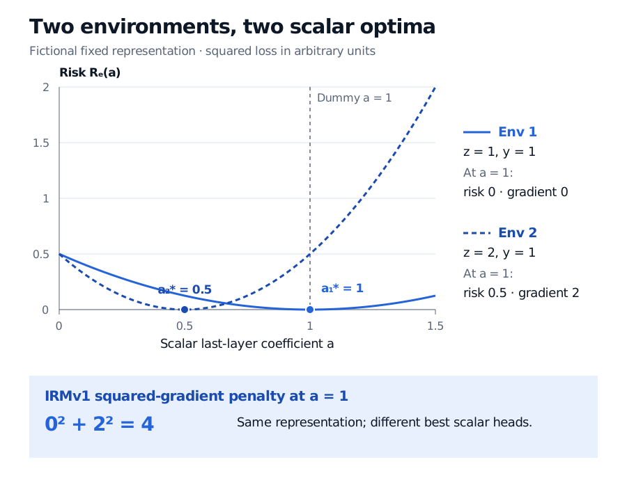
Consider a fictional, deterministic example: hold the representation fixed and restrict the last layer to multiplication by a real scalar a. Environment 1 has represented input z1=1 and target y1=1; environment 2 has z2=2 and y2=1. Define risk as
Re(a)=21(aze−ye)2,dadRe=(aze−ye)ze.
Quantity
Environment 1
Environment 2
Individually optimal scalar
1
0.5
Risk at dummy a=1
0
0.5
Risk derivative at a=1
0
2
No scalar is individually optimal in both environments for this representation. The summed IRMv1 penalty is 02+22=4; its contribution to the objective is 4λ. Using squared error without the one-half factor would change the derivatives and penalty, so the loss convention is part of the calculation.
Fictional scalar-head risks have optima 1 in environment 1 and 0.5 in environment 2. At dummy scalar 1, gradients are 0 and 2, so the summed squared-gradient penalty is 4.
Original deterministic example with a fixed representation and a scalar linear last layer. Risk uses one-half squared error; all quantities are in arbitrary units.
The example tests scalar rescaling only. An unrestricted constant last layer w(z)=1 fits both targets perfectly. It would therefore be wrong to use these two points to prove that the representation fails the full unrestricted IRM constraint.
There is also a cheap way to get a zero scalar penalty: replace both represented inputs by zero. Rescaling zero changes no predictions, so both derivatives vanish. Yet each risk becomes 0.5, and their sum is 1. The prediction-loss term prevents treating the penalty alone as the learning goal. Neither calculation demonstrates that a useful causal feature has been recovered.
The environment choice is part of the claim
A proposed financial application needs a reason why the target relationship should remain stable across its environments. If the same misleading association holds throughout training, environment labels supply little evidence against it. If the economic mechanism itself changes, demanding a shared optimum can discard useful information. These are reasons to inspect environment-specific errors and compare with a simpler pooled model, rather than selecting a penalty solely for its small training gradient.
There are formal failures beyond noisy estimation. In Rosenfeld, Ravikumar and Risteski’s Gaussian classification model, too few informative environments relative to the dimension of environmental features permit constrained solutions that retain those features. Their nonlinear analysis constructs predictors with small training penalties that fail on sufficiently different test environments. These are model-specific counterexamples, not a universal environment-count rule. The Risks of Invariant Risk Minimization, §§3, 5–6
Kamath et al. show a further distinction: scalar/linear invariance can miss full invariance even at population level, and empirical-sample invariance can be fragile. More data cannot automatically repair a mismatch between the surrogate and the intended constraint. Does Invariant Risk Minimization Capture Invariance?, §§3 and 6
For a financial study, environment definitions, feature construction and regularisation strength belong inside the selection procedure. Defining “regimes” after inspecting the final test outcomes spends that test evidence. Time-Ordered Train, Validation and Test Design works through the separation of fitting, selection and confirmation; its preview is public and the full lesson requires membership.
A low IRMv1 penalty is evidence about a specified representation, loss and training environments. It does not identify a causal effect or guarantee performance under every future distribution shift. Causal interpretation needs additional assumptions about how environments are generated and which mechanisms remain unchanged.