Make forecasts across an additive hierarchy agree, work through an equal-weight projection, and distinguish MinT optimality from coherence and probabilistic calibration.
Hierarchical forecast reconciliation
Hierarchical forecast reconciliation adjusts forecasts so that they satisfy the aggregation identities of the underlying data. A forecast of total cash inflows should equal the sum of forecasts for the business units that generate those inflows. Separately fitted models can disagree even when the realised accounting identity is exact. Reconciliation makes the forecast set coherent. Wickramasuriya, Athanasopoulos and Hyndman develop MinT, a method that also uses forecast-error covariance information.
Sharing a discrepancy
Consider fictional cash inflows, in millions of the same currency, for one future month. Business units A and B exhaust the total without overlap. Their independently produced base point forecasts are:
Series
Base forecast
Equal-weight reconciled forecast
Adjustment
Total
100
310/3≈103.3333
+10/3
A
60
170/3≈56.6667
−10/3
B
50
140/3≈46.6667
−10/3
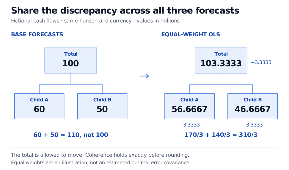
The child forecasts add to 110 while the total forecast says 100. Equal-weight reconciliation lets all three move. It chooses bottom-level values a,b to minimise
(a+b−100)2+(a−60)2+(b−50)2.
The first-order conditions are 2a+b=160 and a+2b=150. Solving gives a=170/3 and b=140/3, so the reconciled total is 310/3. The objective is strictly convex, making this the unique minimum. The adjustment's squared length is 100/3 million-squared; this measures movement from the base forecasts, not error against a future realisation.
Fictional same-horizon cash-flow forecasts in millions: base total 100, child A 60 and child B 50; equal-weight OLS reconciliation gives total 103.3333, A 56.6667 and B 46.6667, coherent before rounding.
Equal-weight reconciliation shares the discrepancy across all three forecasts. Values are shown to four decimals; the fractional values add exactly.
A bottom-up alternative would keep A at 60 and B at 50, replacing the total by 110. Both methods are coherent; they use the aggregate model differently. The forecasting textbook's single-level approaches explain this distinction.
From equal weights to MinT
Write the bottom-level vector as b and all series as y=Sb. Here the summing matrix is
S=110101.
For base forecasts y^h at horizon h, covariance-weighted reconciliation is
y~h=S(STWh−1S)−1STWh−1y^h.
Wh is the covariance matrix of the base forecast errors, not the covariance of observed levels or the adjustments. The displayed inverse formula assumes positive definite Wh and full column rank S. This has the geometry of generalised least squares.
MinT means minimum trace: with unbiased base forecasts, it minimises the sum of reconciled forecast-error variances among linear reconciliation mappings that preserve unbiasedness. Writing the mapping as SG, the preservation condition is SGS=S. These are the conditions behind the optimality statement in Theorem 1 and Section 2.3 of the MinT paper.
Setting Wh=I gives the equal-weight OLS calculation above. No covariance was estimated in that example, so it establishes coherence and projection arithmetic, not empirical optimality. In practice, estimating a large covariance matrix from limited residual history can require shrinkage. Using one-step errors for longer horizons adds a covariance-scaling assumption. Section 2.4 discusses these choices.
For the weighting argument in more detail, the SelfMadeQuant lesson on Generalised Least Squares derives the transformation and explains estimated-weight risks. Its preview is public; the full lesson requires membership.
What must actually add up?
The identity must fit the quantity. Cash flows in a common currency and period can be additive. Percentage returns and rates generally require weights or transformations; summing two business-unit returns does not produce the firm's return. Overlapping groups also require a correctly specified aggregation structure.
Point coherence does not establish a calibrated probabilistic forecast. A joint predictive distribution is coherent when its draws satisfy the identities. Reconcile jointly generated sample vectors, then extract marginal quantiles; preserve the dependence assumptions used to generate those vectors. The textbook's distributional forecast section describes this approach.
Quantiles need not add. Suppose two equally likely outcomes are (A,B)=(0,10) and (10,0), in millions. Total is always 10. Under the inverse-CDF convention, each child's 90th percentile is 10, but the total's 90th percentile is 10, rather than 20. Every outcome is coherent despite the non-additive marginal quantiles. Nor does linear reconciliation automatically enforce non-negativity or integer counts.