Fused lasso and total variation regularisation: Definition & Examples

The fused lasso is a regularised fitting method that penalises both coefficient magnitudes and differences between neighbouring coefficients. The difference penalty can make neighbours exactly equal. For a quant modelling a noisy exposure profile across maturities, this offers a way to estimate stretches of a common level while retaining jumps between them.

The original method combines ordinary L1 regularization, which encourages zero coefficients, with fusion, which encourages zero differences. These are separate modelling choices. Tibshirani and co-authors (2005), §2, introduce the two constraints; §4 gives the penalised formulation.

Two penalties, two kinds of sparsity

For an ordered coefficient vector, one least-squares convention is

\min_{\boldsymbol{\beta}}\left\{ \frac12\sum_{i=1}^{n}\left(y_i-\sum_{j=1}^{p}x_{ij}\beta_j\right)^2 +\lambda_1\sum_{j=1}^{p}\lvert\beta_j\rvert +\lambda_{\mathrm{TV}}\sum_{j=2}^{p}\lvert\beta_j-\beta_{j-1}\rvert \right\}.

Here

y_i

is the response,

x_{ij}

the design, and both penalty weights are nonnegative. An intercept may be fitted separately without penalisation; none is included in this displayed convention. The final sum is discrete total variation along the chosen chain. It measures the aggregate size of changes, rather than counting them.

The coefficient penalty favours sparse levels; the TV penalty favours sparse changes, creating piecewise constant profiles. Replacing absolute differences by squared differences gives a different smoother, without the same kink that permits exact fusion.

In signal denoising, each observation has its own fitted level: the design is the identity and

p=n

. Setting

\lambda_1=0

gives one-dimensional total variation denoising, also often called the one-dimensional fused lasso. This naming convention is explicit in Madrid Padilla and co-authors, equations (2) and (7). TV-only denoising does not itself ask for the fitted levels to be zero.

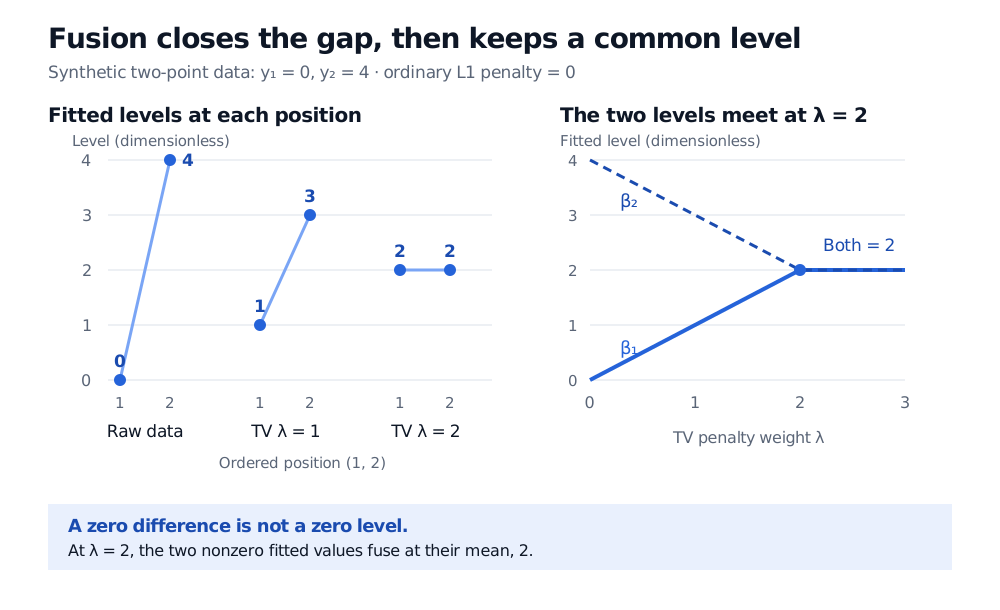
Watch two observations fuse

Take synthetic dimensionless observations $y_1=0$ and $y_2=4$ . Use the TV-only objective, with no averaging of the squared loss:

J(\beta_1,\beta_2) =\frac12\left[\beta_1^2+(\beta_2-4)^2\right] +\lambda_{\mathrm{TV}}\lvert\beta_2-\beta_1\rvert.

While $\beta_2>\beta_1$ , setting the two derivatives to zero gives $\beta_1=\lambda_{\mathrm{TV}}$ and $\beta_2=4-\lambda_{\mathrm{TV}}$ . They meet when $\lambda_{\mathrm{TV}}=2$ .

TV weight	Fitted levels	Squared-error loss	TV penalty	Full objective
$1$	$(1,3)$	$1$	$2$	$3$
$2$	$(2,2)$	$4$	$0$	$4$

At weight one, keeping the raw observations gives objective four, and forcing both levels to two also gives four. The intermediate fit wins with three. At weight two, the optimum is fully fused, but both levels remain nonzero.

Why do they stay fused beyond that point? At equal levels, the absolute difference has a subgradient $s\in[-1,1]$ . Optimality requires

\beta_1-\lambda_{\mathrm{TV}}s=0, \qquad \beta_2-4+\lambda_{\mathrm{TV}}s=0.

The common level two satisfies both conditions with $s=2/\lambda_{\mathrm{TV}}$ whenever $\lambda_{\mathrm{TV}}\geq2$ . The objective is strictly convex, so these conditions identify its unique minimiser. A further increase in the TV weight cannot lower the difference below zero.

Synthetic observations zero and four become fitted levels one and three at TV lambda one, then two and two at lambda two. The fitted-level paths meet at two and remain there as lambda increases.

Original dimensionless example with ordinary L1 penalty set to zero. Solid and dashed paths identify the first and second fitted levels; the TV penalty fuses their difference without shrinking the common level to zero.

These numerical weights belong to the displayed half-sum loss. Averaging that loss over observations changes the penalty scale needed for the same fit.

Neighbourhood and information timing matter

Adjacency is part of the model. A maturity order has a different meaning from an arbitrary alphabetical ordering of assets. For a graph, the analogous TV penalty sums absolute fitted differences over specified edges, as defined in Madrid Padilla and co-authors, §1. Changing those edges changes which values are encouraged to agree. If a neighbourhood is learned from data, estimate it within the training sample.

The quant application also needs an information boundary. Fitting a whole historical time series jointly can use observations after date $t$ to estimate the fitted level at $t$ . The two-point example already demonstrates this: the estimate for the first position changes from zero to one because the second observation is included. A retrospective denoising curve is therefore not automatically a causal forecast or an available trading signal.

For a predictive backtest, recreate each fit using only information available at its decision time, and select penalty settings using a validation scheme that respects that timing. Otherwise smoothing can introduce preprocessing leakage. Even a correctly timed fit expresses a preference for locally constant levels; its jumps do not by themselves establish economic regimes or statistically confirmed structural breaks.

For the baseline distinction between penalties on coefficient magnitudes, see Ridge, Lasso, and Elastic Net (membership; public preview).

Sources

Tibshirani, Saunders, Rosset, Zhu and Knight (2005), Sparsity and smoothness via the fused lasso, JRSS B, 67(1), 91–108, §2 and §4 equation (6): coefficient sparsity, fusion and the two-penalty formulation.
Madrid Padilla, Sharpnack, Scott and Tibshirani, The DFS Fused Lasso: Linear-Time Denoising over General Graphs, §1 equations (2) and (7): graph total variation and its one-dimensional chain special case.

Two penalties, two kinds of sparsity

Watch two observations fuse

Neighbourhood and information timing matter

Sources

Related terms

L1 regularization