Factor alignment problem: Definition & Examples

The factor alignment problem arises when a portfolio's return forecasts contain directions that its risk model does not represent as common factors. An optimizer can then concentrate on those directions because they appear to offer return for little modelled risk. The practical problem is the interaction between the alpha forecast, the risk model and portfolio constraints, rather than a large factor exposure by itself.

For example, two momentum signals can use almost the same history yet disagree at the beginning or end of the lookback. Optimizing one against a risk model built from the other can turn that small definitional difference into a large position. MSCI's 2016 research preview describes the resulting unintended exposures and trading; the full paper requires a contact-information form.

What sits outside the risk-factor space?

Let $B$ be an asset-by-factor exposure matrix and write the model covariance matrix as

\Sigma_m=BFB^\top+D,

where $F$ is factor-return covariance and $D$ is specific-return covariance. The risk-factor space is the set of asset-level vectors obtainable as $Bc$ for some vector $c$ .

For a full-column-rank $B$ , an ordinary Euclidean projection decomposes the expected-return forecast $\alpha$ into

\begin{aligned} P_B&=B(B^\top B)^{-1}B^\top,\\ \alpha_\parallel&=P_B\alpha,\\ \alpha_\perp&=(I-P_B)\alpha. \end{aligned}

Here

B^\top\alpha_\perp=0

. The residual forecast is orthogonal to the model's factor-exposure columns in this chosen cross-sectional geometry. It need not be statistically independent of factor returns, and it need not be a return-series regression intercept. Weighted projections use a different geometry and must state their weights.

Outside the factor space does not mean outside the entire risk model:

D

still assigns risk. Nor does it mean the residual forecast is worthless. The Karels–Sun chapter, §§24.3–24.5, distinguishes residual noise from residual forecasts that may carry both useful return information and additional risk.

A spread the optimizer regards as cheap

Consider a fictional two-asset target portfolio. All forecasts refer to the same single period, with simple returns expressed as decimals and covariance entries in squared decimal-return units. The period is deliberately unspecified; none of the figures is annualized. Weights are signed notionals divided by a common capital base.

The model contains one common factor with loading $B=(1,1)^\top$ , variance $0.009$ , and specific covariance $D=0.001I$ . Thus

\Sigma_m= \begin{pmatrix} 0.010&0.009\\ 0.009&0.010 \end{pmatrix}, \qquad \alpha=\begin{pmatrix}0.02\\-0.02\end{pmatrix}.

The forecast likes A and dislikes B. It is entirely orthogonal to the common loading: $B^\top\alpha=0$ . Choose the synthetic mean–variance optimization objective

\max_{w\in\mathbb{R}^2}\; \alpha^\top w-\frac{10}{2}w^\top\Sigma_mw.

This is an unconstrained target: there is no fully invested budget requirement, leverage cap, short-sale restriction, financing cost or turnover penalty. The parameter

10

is an illustrative risk penalty in these return units. It is not a calibrated investor preference or a recommended allocation.

Since $\Sigma_m$ is positive definite, the first-order condition gives the unique maximum:

w^*=\frac1{10}\Sigma_m^{-1}\alpha =\begin{pmatrix}2\\-2\end{pmatrix}.

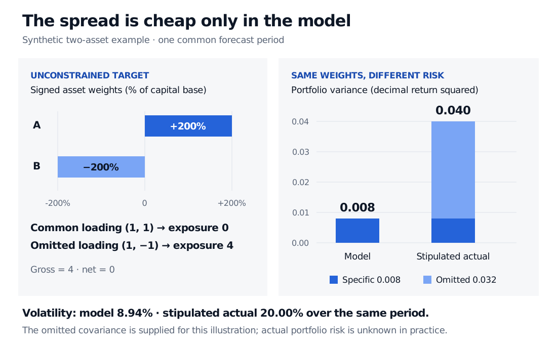
That is long 200% in A and short 200% in B: gross exposure $4$ , net exposure $0$ . The common factor cancels, $B^\top w^*=0$ , so the model charges only specific variance:

(w^*)^\top\Sigma_mw^*=0.001(2^2+(-2)^2)=0.008.

Now stipulate, solely for this example, an omitted spread factor with loading

b=(1,-1)^\top

, variance

0.002

, and zero covariance with the modelled factor and specific returns. The synthetic actual covariance is

\Sigma_a=\Sigma_m+0.002bb^\top =\begin{pmatrix} 0.012&0.007\\ 0.007&0.012 \end{pmatrix}.

The same holdings have omitted-factor exposure $b^\top w^*=4$ , giving

\begin{aligned} (w^*)^\top\Sigma_aw^* &=0.008+0.002(4)^2\\ &=0.040. \end{aligned}

Modelled volatility is $\sqrt{0.008}\approx8.94\%$ ; stipulated actual volatility is $\sqrt{0.040}=20\%$ over that same period. The variance is five times the forecast, while volatility is about 2.24 times the forecast. Those ratios differ because volatility is the square root of variance.

Synthetic unconstrained weights are plus 200 percent in A and minus 200 percent in B, giving common-factor exposure zero and omitted-spread exposure four. Model variance is 0.008; stipulated actual variance is 0.040, including 0.032 of omitted-factor variance.

Original synthetic example. Zero exposure to the modelled common factor does not eliminate an omitted spread driver. Variances use decimal-return-squared units over one common forecast period.

The discrepancy follows from the covariance we supplied. In a real portfolio, actual future covariance is unknown. Orthogonality alone does not establish that an omitted factor exists, measure its variance, or prove that every residual alpha is dangerous. If the spread truly had only the modelled specific risk, this particular risk understatement would disappear.

Diagnose the mismatch before choosing a response

First inspect the projected and residual forecasts alongside the positions the optimizer actually chooses. A small residual forecast can matter if the model assigns very little variance to its direction. Compare factor definitions, asset universes, signal timing and forecast horizons; nominally identical factor names do not establish identical exposures.

Then investigate whether the residual direction has persistent common return variation, unstable predictive content, or mainly stock-specific variation. Evaluate the resulting portfolios out of sample, including their realized risk and trading. A projection is a diagnostic decomposition, not an estimator of omitted-factor risk.

Possible responses include estimating a risk model that incorporates the relevant additional drivers, adding a targeted residual-exposure penalty, or rescaling the residual forecast. Their suitability depends on what the residual represents. MSCI's public author summary discusses these alternatives; its comparisons concern particular research settings, not a universal ranking. Removing a risk factor simply because it clashes with an alpha signal can also remove genuine risk information.

Constraints matter as well. Position limits can contain an extreme spread, while benchmark, sector or trading constraints change which directions the optimizer can reach. Saxena and Stubbs' published abstract explicitly treats the interaction of expected returns, constraints and the risk model. An unconstrained calculation isolates the mechanism; it does not describe every production portfolio.

A different issue from matching factor labels

Changing the sign of a factor and its loading together preserves fitted returns. More generally, replacing $B$ by $BA$ for an invertible matrix $A$ leaves its column space unchanged; transforming factor covariance to $A^{-1}FA^{-\top}$ also preserves $BFB^\top$ . Such basis changes do not remove $\alpha_\perp$ or repair omitted covariance.

Matching signs, rotating latent factors across estimation windows, and deciding whether a PCA component has a stable economic interpretation are identification and comparison questions. The factor alignment problem here concerns whether the alpha and risk spaces support a coherent portfolio construction decision.

For the mechanics, Mean–Variance Optimisation and Portfolio Theory derives the inverse-covariance solution, while Risk Models, APT and Factor Structure explains common and specific covariance. Both have public previews; full lessons require membership.

Sources

Bayraktar, Melas and Roisenberg (2016), Are Your Factors Aligned?, MSCI. Public research preview; full paper is form-gated. The accompanying public blog by Bayraktar summarizes the mechanism and alternative responses.
Karels and Sun (2013), Active Portfolio Construction When Risk and Alpha Factors Are Misaligned, Chapter 24 of Rethinking Valuation and Pricing Models, especially §§24.3–24.5. Public MSCI-hosted chapter.
Saxena and Stubbs (2013), The Alpha Alignment Factor: A Solution to the Underestimation of Risk for Optimized Active Portfolios, Journal of Risk 15(3). Publisher abstract read; full article requires access.