Trace a two-way merge and see how the master theorem turns the cost of each recursive call into the running time of a full merge sort.
Divide and conquer and the master theorem
Divide and conquer is an algorithm design strategy. Split a problem into smaller instances of the same problem, solve them using recursion until a base case is reached, and combine the answers. The master theorem gives the time complexity for a class of recurrences that arise from this strategy. In a backtest that ingests batches of market events, merge sort illustrates both ideas. Sorting batches separately is useful because the resulting ordered runs can be stitched together with a single pass.
Two sorted runs, one pass
Take two fictional runs of event timestamps, measured in milliseconds from the same origin. The left run contains 2, 5, 9, 13 and the right contains 1, 6, 10, 12. To merge them, compare the first unread value in each run. The smaller one is the smallest remaining value overall because both runs are already sorted. Write it to the output and advance only its run. Once either run is empty, append the remainder of the other run in order.
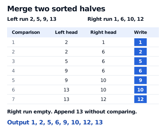
Two sorted runs, 2, 5, 9, 13 and 1, 6, 10, 12, merge in seven head comparisons. The right run is then empty, so 13 is appended without comparison. The output is 1, 2, 5, 6, 9, 10, 12, 13.
The blue column shows which value each comparison writes. The last value needs no head comparison.
Seven comparisons suffice here because the right run runs out just after 12 is written. Across two nonempty runs with n items in total, there are at most n−1 head comparisons. At least one item is left when the first run empties. Writing every item still takes Θ(n) time when comparing and writing each record costs constant time. For real event records, the runs must use the same ordering key. If the timestamp alone leaves simultaneous events tied, specify the tie order the backtest needs.
From the last merge to the full sort
The example starts with sorted halves and shows only the combine step. A standard top-down merge sort starts with arbitrary input. It divides the input in half, sorts both halves recursively, then merges them. An empty run or a run with one item is already sorted. With n a power of two, a constant-time base case, and linear work outside the recursive calls, the running time obeys
T(n)=2T(n/2)+Θ(n).
At depth i there are 2i runs of size n/2i. The work outside the recursive calls adds up to Θ(n) at each merge level. There are log2n such levels, so the full sort takes Θ(nlogn) time. For other input sizes, the two calls use the floor and ceiling of n/2. The splits remain balanced and the same bound holds. MIT 6.006, Lecture 3
What the master theorem compares
In the clean equal-size case, write T(n)=aT(n/b)+f(n), where a≥1 is a fixed number of recursive calls, b>1 is a fixed shrink factor and f(n)≥0 counts all work outside those calls, including dividing and combining. For n=bk with integer b and k, and a base case T(1)=Θ(1), there are np leaves, where p=logba. The basic three cases compare f(n) with that leaf count. MIT 6.006, Recitation 3
Work per call
Total time
f(n)=O(np−ε) for some ε>0
Θ(np)
f(n)=Θ(np)
Θ(nplogn)
f(n)=Ω(np+ε) for some ε>0, with af(n/b)≤cf(n) for a constant 0<c<1 and all sufficiently large n
Θ(f(n))
Merge sort lands in the middle case because a=b=2 and f(n)=Θ(n). The first and third cases require a polynomial gap. A logarithmic factor alone does not establish either case. Count the recursive calls and the work each one does before applying a bound. A recurrence with unequal sizes, such as T(n/3)+T(2n/3)+f(n) on the right-hand side, falls outside this equal-size form. A recursion tree lets you track the cost of its branches directly.
For a different combine step, the SelfMadeQuant design-paradigms lesson shows how to aggregate P&L across independent backtest runs. The full lesson requires membership.