A depthwise separable convolution is a convolutional block that filters each input channel independently, then combines the filtered channels with a pointwise convolution. It reduces the number of learned weights and arithmetic operations relative to an ordinary convolution, at the cost of constraining how spatial and channel relationships interact. For a quant model processing grid-shaped market features, this can make a smaller convolutional neural network worth testing when memory or inference time is limited; it does not establish predictive usefulness.
Filter first, mix second
An ordinary convolution learns a spatial filter for every input–output channel pair and adds their contributions. A depthwise separable block splits the work:
- Depthwise: apply a spatial filter separately to each input channel. With depth multiplier one, four input channels produce four filtered channels. No information passes between channels at this stage.
- Pointwise: apply a convolution to combine those filtered values into the desired output channels. “One by one” describes the spatial footprint; the operation can use every filtered channel.
This is the construction in MobileNets §3.1. A channel is a feature dimension, such as separate measurements at each grid location, rather than another spatial position.
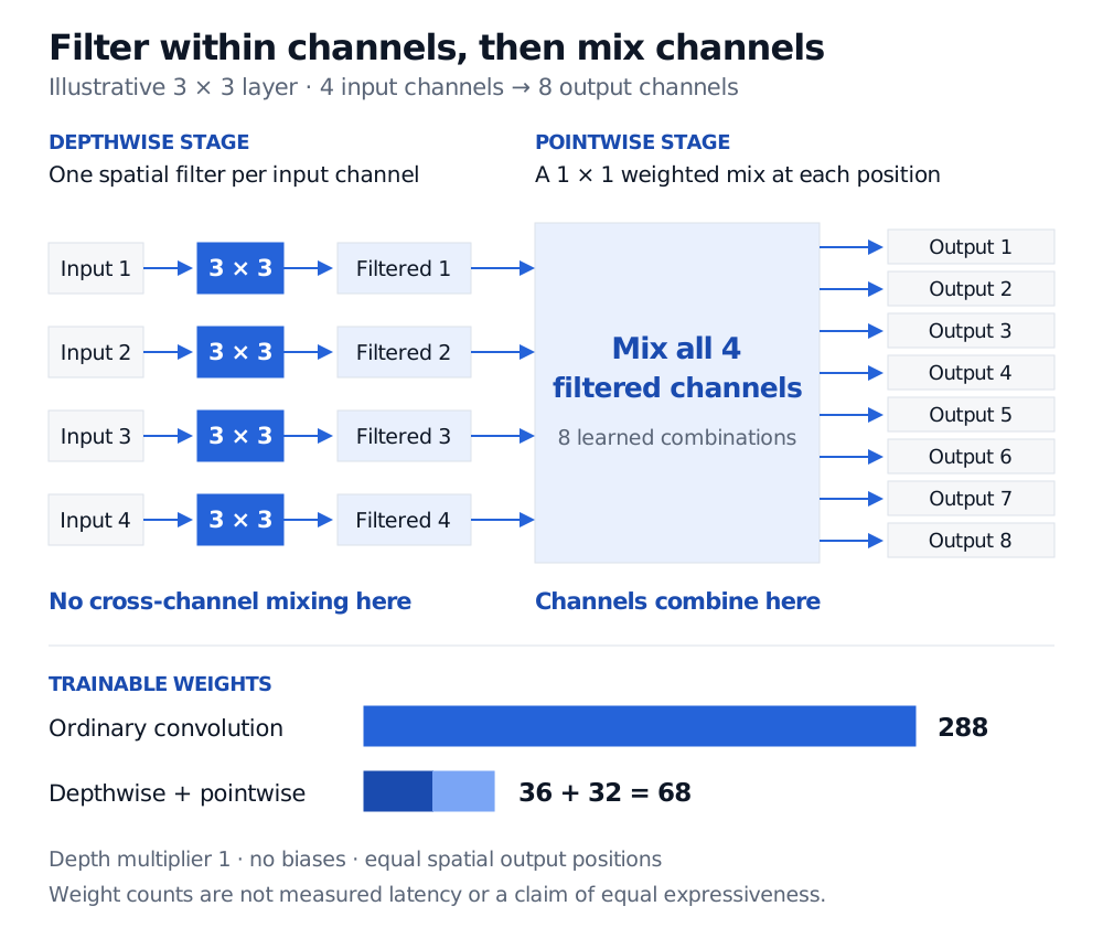
Original illustrative architecture: mixing occurs in the pointwise stage. Counts exclude biases and use depth multiplier one.
Where the 68 weights come from
Take a kernel, four input channels and eight output channels. Use depth multiplier one, exclude biases and normalisation parameters, and compare the same spatial output positions.
| Construction | Learned weights | Count |
|---|---|---|
| Ordinary convolution | Nine spatial weights for each of 4 × 8 channel pairs | 288 |
| Depthwise stage | Nine spatial weights for each of four input channels | 36 |
| Pointwise stage | Four input weights for each of eight output channels | 32 |
| Depthwise + pointwise | Both stages together | 68 |
For square kernel width , input channels and output channels , the bias-free counts are
Our example retains of the weights, or about 76.4% fewer. Counting one multiply–accumulate per weight per output position gives the same ratio of arithmetic counts under these assumptions. The general ratio is .
The ratio is not a promise of 4.24 times lower latency. Memory traffic, intermediate activations and the implementation of each operation also matter. MobileNets §3.2 explicitly distinguishes arithmetic counts from efficient implementation; Xception §4.5.2 also reports speed separately from parameter count.
The saving imposes a restriction
Consider the two stages without any activation or other intervening transformation. Let be the depthwise filter and the pointwise weight. Their effective ordinary-convolution kernel must satisfy
For one fixed input channel, every output channel therefore sees a scalar multiple of the same spatial pattern. An unrestricted ordinary convolution can use a different pattern for each output. For example, it can read only the top-left entry for one output and only the top-middle entry for another, from that same input channel. Those two patterns are not scalar multiples, so this multiplier-one linear block cannot represent them both.
A larger depth multiplier supplies more spatial filters per input channel and changes both the count and the restriction. Nonlinearities between stages change the function again: the kernel identity above applies only to the linear composition. Activation placement is a separate design choice. MobileNets uses normalisation and ReLU around its stages, while Xception §4.7 investigates intermediate activations and uses none in its main separable operation. Neither architecture makes a separable block universally interchangeable with an ordinary layer.
Two nearby ideas to keep separate
Spatial separability factors the spatial axes, for example a operation followed by a operation. Depthwise separability separates spatial filtering from channel mixing. A depthwise filter need not itself factor into two one-dimensional filters. Xception §1.2 makes this distinction explicitly.
Grouped convolution partitions channels into groups. Depthwise filtering is the extreme grouping case, with one input channel per group; a general grouped convolution can still mix several input channels inside each group. The depthwise stage alone is only part of the separable block: the following pointwise stage restores mixing across channels. The PyTorch Conv2d reference describes these group connectivity rules.
For background on shared filters, stride and padding, Convolutional Networks for Structured Data develops the ordinary CNN construction. Its preview is public; the full lesson requires membership.
Sources
- Howard et al. (2017), MobileNets: Efficient Convolutional Neural Networks for Mobile Vision Applications, §§3.1–3.2: separate filtering and mixing, computational counts and implementation considerations.
- Chollet (2017), Xception: Deep Learning with Depthwise Separable Convolutions, §1.2 and §§4.5.2, 4.7: channel-versus-spatial separation, measured speed and intermediate activation choices.
- PyTorch, Conv2d reference: groups: full, grouped and depthwise channel connectivity.