A surrogate loss is classification-calibrated when its population optimum recovers the Bayes decision boundary. See why log loss and hinge loss qualify, while only the former identifies the class probability.
Classification-calibrated surrogate loss
A classification-calibrated surrogate loss is a training loss function whose best population risk is strictly better than any score on the wrong side of the optimal classification boundary. It justifies replacing the discontinuous 0–1 classification loss with a more tractable objective. For a quant predicting a binary event, this connects the training target to classification error; it does not establish profitable trades or trustworthy sizing probabilities.
What must the population optimum get right?
Take labels Y∈{−1,+1}, a real score a=f(x) and equal costs for the two kinds of classification error. Write η=P(Y=+1∣X=x). The Bayes decision predicts +1 when η>1/2 and −1 when η<1/2. At η=1/2, either label has the same error.
For a nonnegative margin loss ϕ(Ya), define its conditional risk and two infima:
Classification calibration requires H−(η)>H(η) whenever η=1/2. The constrained infimum includes a zero score, so the condition rules out approaching the optimum by sitting on the boundary as well as choosing the wrong sign. Infima also cover losses whose optimum is approached only at an infinite score. This is the definition in Bartlett, Jordan and McAuliffe, §2.2.
Log loss: the correct sign comes with a probability target
Consider a specified population, not a fitted backtest: at one feature value, η=0.7. Predicting +1 has conditional error 0.3; predicting −1 has error 0.7. Choosing the wrong class costs an extra 0.4 in expected 0–1 loss.
Let q∈(0,1) be the predicted positive-label probability. With natural logarithms, expected log loss is
The derivative changes from negative to positive at q=η. Thus the unique minimum is q∗=0.7:
Probability prediction
Expected log loss
Classification implication
q=0.7
0.610864
Correct side and population optimum
q=0.5
0.693147
Decision boundary; tie rule needed
q=0.4
0.794651
Wrong side
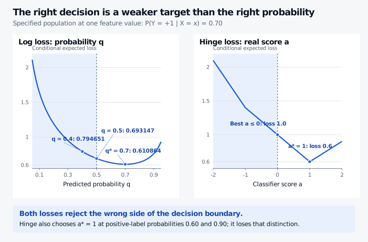
The best prediction constrained to q≤0.5 is the boundary, leaving a strictly positive loss gap of 0.082283. Under the logit score a=log(q/(1−q)), this is exactly the constraint a≤0. The unconstrained optimum is a∗=log(0.7/0.3)≈0.847298, which has the Bayes sign.
At a specified positive-label probability of 0.7, log loss is minimised at q equal to 0.7 with loss 0.610864. At q equal to 0.5 loss is 0.693147; at q equal to 0.4 it is 0.794651. Hinge risk is minimised at score 1 with loss 0.6; the best nonpositive score has loss 1.0.
Original population-risk illustration, with separate probability and score axes. Both losses favour the correct class; the hinge optimum does not identify the positive-label probability.
Hinge: enough information for a class, less than a probability
The support vector machine uses hinge loss ϕ(Ya)=max(0,1−Ya). At η=0.7, its conditional risk is
C0.7(a)=0.7max(0,1−a)+0.3max(0,1+a).
On −1≤a≤1, this becomes 1−0.4a. It decreases until a=1 and increases thereafter. Its minimum is 0.6; the best nonpositive score is a=0, with loss 1. Hinge is classification-calibrated, as Bartlett and co-authors show in Example 4.
But η=0.6 and η=0.9 also produce the same optimal hinge score a∗=1. That score cannot tell those probabilities apart. Simply rescaling it or applying a sigmoid cannot recover information the optimum has discarded.
Three meanings that must stay separate
Classification calibration targets the Bayes class at the stated decision threshold. Strict properness targets the true probability as the unique conditional-risk minimiser: log loss has this property. Hinge, a score loss, is not a proper probability loss under the simple probability encoding a=2q−1: for η=0.7, it prefers q=1 to q=0.7. Reid and Williamson, §§3.1 and 5, distinguish these loss properties.
Probability calibration asks whether forecast probabilities match outcome frequencies conditional on the forecast. Classification calibration alone does not imply that reliability; neither does fitting a finite sample with a strictly proper loss.
For a calibrated margin loss, convergence of population surrogate risk to its infimum over all measurable scores implies convergence to Bayes 0–1 risk (Bartlett et al., Theorem 1). A low training loss does not establish that premise: finite data, optimisation error, regularisation and a misspecified function class can leave population excess risk. Changing the deployment distribution introduces another gap. Unequal error costs require a different decision threshold; equal-cost classification calibration does not certify an economic trading objective.