The underlying share buyback is a corporate transaction. Announcement drift is a return pattern around news of that transaction. A board authorisation describes permission or intention to repurchase; it does not establish that the company has bought the announced amount. Nor is this post-earnings-announcement drift: the event here is repurchase news, rather than an earnings surprise. If both arrive together, their effects are difficult to separate.
Start the clock after the news
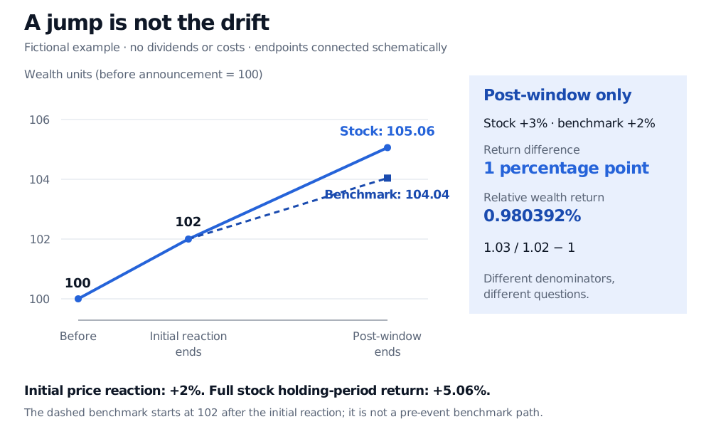
Consider a fictional stock with no dividends over the example. Its price is 100 immediately before the announcement reaction and 102 at the end of that initial reaction: a 2% price increase. Over a separately specified post-announcement holding window, the stock returns 3% and a benchmark returns 2%.
The stock finishes at . Investing the same 102 in the benchmark at the start of the post-announcement window would finish at . These are different questions:
| Measurement | Result | What it includes |
|---|---|---|
| Initial stock price reaction | 2% | The move from 100 to 102 |
| Post-window stock return | 3% | The move from 102 to 105.06 |
| Post-window return difference | 1 percentage point | Stock 3% minus benchmark 2% |
| Full stock holding-period return | 5.06% | Both the initial reaction and later return |
For a multiday window, the conventional difference-form buy-and-hold abnormal return is
It expresses the wealth advantage relative to ending benchmark wealth. State the convention explicitly; the two quantities use different denominators. Neither should be silently substituted for a cumulative abnormal return, which adds period-by-period abnormal returns rather than taking a difference of compounded wealth paths.
An actual research design must also define what “after” means. If news arrives after the exchange closes, an entry at that same closing price uses information that was unavailable at the assumed trade. Preserve the public release timestamp, time zone and revisions; define the reaction window and a feasible entry before measuring the subsequent window. A daily event label alone does not establish an executable price.
Why researchers looked beyond the announcement jump
Turn the headline into a testable event
A useful event study specifies the announcement population, return window and benchmark together. Several choices can otherwise manufacture an appealing result:
- Authorisation versus execution. Define whether events are new programmes, increases, renewals or another transaction type. Do not select only programmes later known to be completed if the proposed signal is the announcement. Subsequent executed repurchases are a separate, later information set.
- Benchmark and sample selection. A broad market index may leave size, value, industry or other exposures in the result. Compare suitable matched firms or factor models using characteristics available at formation. Keep delisted firms and their terminal returns; dropping failures creates survivorship bias.
- Overlapping observations. Repeated announcements from one issuer can count the same later returns several times. Programmes also cluster across firms in the same market conditions. Define treatment of repeats and use inference that respects dependence, with calendar-time portfolio analysis as a useful complementary design.
- Trading economics. A gross benchmark-adjusted return is not net profit. Entry delay, spreads, market impact, turnover and any hedge's financing or borrow costs belong in a separate executable portfolio test. Specify weights and holding rules, then test them on later data without retuning to the result.
Long horizons compound both returns and benchmark errors. Managers also choose when to announce, and announcements can coincide with earnings, financing changes or other news. A positive association therefore does not identify the causal effect of repurchasing shares. It may reflect delayed information processing, imperfect risk adjustment, selection or several mechanisms together.
Sources
- Ikenberry, D., Lakonishok, J. and Vermaelen, T. (1995). Market underreaction to open market share repurchases. Journal of Financial Economics, 39, 181–208. Published abstract supports the historical 12.1% result.
- Ikenberry, D., Lakonishok, J. and Vermaelen, T. (December 1993). Earlier INSEAD working-paper version, introduction, data and methodology. Its numerical estimates differ from the final published abstract.
- Peyer, U. and Vermaelen, T. (2009; online 2008). The Nature and Persistence of Buyback Anomalies. Review of Financial Studies, 22(4), 1693–1745. Abstract.
- Mitchell, M. L. and Stafford, E. (2000). Managerial Decisions and Long-Term Stock Price Performance. Journal of Business, 73(3), 287–329, introduction and section III.