Binary lifting: Definition & Examples

Binary lifting answers ancestor queries on a rooted tree by storing jumps of length 1, 2, 4, 8 and so on. A risk reporting service can use it to look up which reporting unit is exactly

k

levels above a trading book, even when it has to answer many such queries against the same hierarchy.

Build each jump out of two shorter ones

Every node except the root has one parent. Write $p(v)$ for the parent of node $v$ , and let $J_j(v)$ be the node reached by climbing exactly $2^j$ edges from $v$ . The first entry is the parent. Each longer entry follows two jumps of half the length.

J_0(v)=p(v),qquad J_{j+1}(v)=J_j(J_j(v)).

This is a bottom-up dynamic program. Compute all one-edge entries, then all two-edge entries, then all four-edge entries. Each new entry uses only the previous column, so the order of the node IDs is irrelevant.

Use $-1$ to mean that an ancestor is missing, and propagate it through all longer jumps. A request for zero edges returns the starting node. A request for exactly the node's depth reaches the root, and any larger request returns $-1$ .

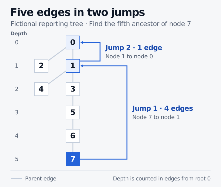
The fifth ancestor of node 7

Take a fictional hierarchy with node IDs 0 through 7 and parent array $(-1,0,0,1,1,3,5,6)$ in that order. Node 0 is the root. A few rows of the jump table show how the query works.

Starting node	1 edge	2 edges	4 edges
7	6	5	1
5	3	1	$-1$
1	0	$-1$	$-1$
0	$-1$	$-1$	$-1$

The four-edge entry for node 7 combines the two-edge jump from 7 to 5 with the two-edge jump from 5 to 1. A five-edge query uses

5=4+1

. It first jumps from 7 to 1, then takes the one-edge entry for node 1, reaching 0. The one-edge entry for node 7 would take you to 6.

In the fictional tree, the parent chain is 7 to 6 to 5 to 3 to 1 to 0. Jump 1 climbs four edges from 7 to 1. Jump 2 climbs one edge from 1 to root 0, the fifth ancestor of 7.

The two arrows show the lookups in query order. Depth is measured in parent edges from the root.

A six-edge query on node 7 goes past the root. In Python, guard the sentinel before using it as an index. A lookup at index -1 would read the last element of the row and could turn a missing ancestor into an ordinary node ID.

Query the set bits

The code assumes a valid, nonempty rooted tree with IDs from 0 through $n-1$ , a valid starting node and an integer $k\ge 0$ . The largest possible climb is $n-1$ edges, so the table only needs enough columns to represent that distance. The query checks the bits of $k$ from largest to smallest and takes the corresponding jump each time it finds a 1.

def build_jumps(parents: tuple[int, ...]) -> list[list[int]]:
    """Store jumps by power, then by node."""
    jumps = [list(parents)]
    columns = max(1, (len(parents) - 1).bit_length())
    for _ in range(1, columns):
        shorter = jumps[-1]
        jumps.append([shorter[middle] if middle != -1 else -1 for middle in shorter])
    return jumps


def kth_ancestor(jumps: list[list[int]], node: int, k: int) -> int:
    """Climb k parent edges and return -1 if the ancestor is missing."""
    bits = k.bit_length()
    if bits > len(jumps):
        return -1
    for power in range(bits - 1, -1, -1):
        if (k >> power) & 1:
            node = jumps[power][node]
            if node == -1:
                return -1
    return node


jumps = build_jumps((-1, 0, 0, 1, 1, 3, 5, 6))
print(kth_ancestor(jumps, 7, 5))
# 0
print(kth_ancestor(jumps, 7, 6))
# -1
print(kth_ancestor(jumps, 7, 0))
# 7

For $n$ nodes, this table takes $O(n\log n)$ time to build and space to store. It answers each query in $O(\log n)$ time under constant-time array access and word operations. A direct walk can be cheaper for a few queries on a shallow tree. Reuse the table across queries on a fixed hierarchy, and rebuild it if parent links change. If a book can report to several parents, specify which parent relation to follow before asking for a unique ancestor.

The same jump table can bring two nodes to equal depth before finding their lowest common ancestor. In a reporting tree, that common ancestor identifies the smallest reporting unit that contains both books.

If your tree arrives as an edge list, the SelfMadeQuant lesson Breadth-First and Depth-First Search shows how a traversal from the root records a parent and an edge count for each node. The public page is a preview. The full lesson requires membership.

Sources

Michael A. Bender and Martín Farach-Colton analyse power-of-two ancestor pointers and their running time in Section 3.2. The Level Ancestor Problem Simplified
Antti Laaksonen covers finding an ancestor through powers of two in Section 18.1 and using the same table for common ancestors in Section 18.3. Competitive Programmer’s Handbook

Build each jump out of two shorter ones

The fifth ancestor of node 7

Query the set bits

Sources

Related terms

Dynamic programming

Lowest common ancestor