Bertsimas–Lo execution model: Definition & Examples

The Bertsimas–Lo execution model chooses how to divide a fixed stock order across a finite number of trading periods to minimise expected purchase cost. Its practical contribution is to treat optimal execution as a sequence of decisions: today's trade changes both the remaining order and the prices faced later. Bertsimas and Lo's 1998 paper solves this problem with stochastic dynamic programming.

Equal slices emerge from one particularly simple specification. That result is useful precisely because its assumptions can be written down and tested; it does not establish that a time-weighted schedule is generally optimal.

The price paid includes this trade's impact

Consider a buy programme for $X$ shares completed in $T$ equal-duration periods. Write $S_t$ for shares bought in period $t$ , with

S_t\ge0,\qquad \sum_{t=1}^{T}S_t=X.

Use the paper's basic price law, Eq. (2.3):

P_t=P_{t-1}+\theta S_t+\varepsilon_t,\qquad \theta>0.

Here

P_t

is the execution price paid for every share in that period, after the order's own linear market impact. It also becomes the next period's starting price, so this impact is permanent within the model. Prices and shocks have units USD per share;

\theta

has units USD per squared share, making

\theta S_t

a price increment.

At the start of period $t$ , choose $S_t$ using information $\mathcal F_{t-1}$ already available, before observing $\varepsilon_t$ . Assume independent, integrable, zero-mean shocks, independent of that information, so $\mathbb E[\varepsilon_t\mid\mathcal F_{t-1}]=0$ . Trades cannot anticipate future shocks. The objective is

\min_{\{S_t\}}\mathbb E\left[\sum_{t=1}^{T}P_tS_t\right].

This is a risk-neutral cash-cost objective. There is no separate variance penalty, spread, fee, participation cap or partial-fill process here. Completion is required on every path, and quantities are divisible. The paper initially omits the no-sales constraint; we impose nonnegative buys, which its basic solution satisfies anyway.

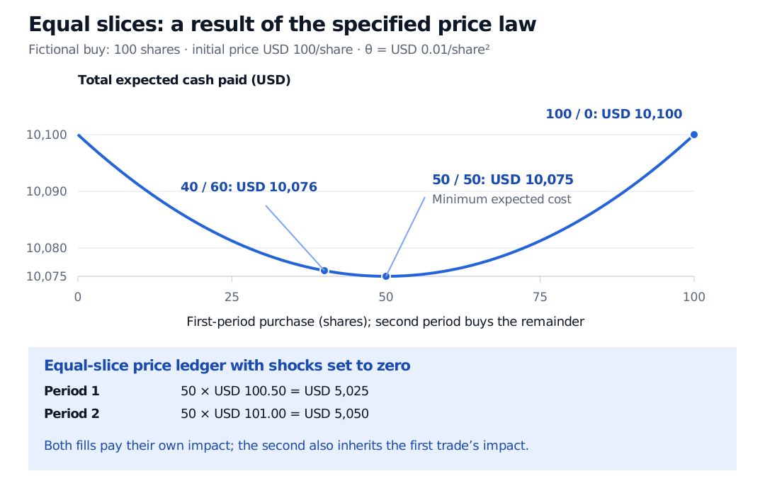
Take fictional inputs $P_0=100$ , $X=100$ , $T=2$ and $\theta=0.01$ . Set shocks to zero for the displayed price ledger. These deterministic schedules have the same expected costs with the stated zero-mean shocks.

Buys in periods 1 and 2 (shares)	Period-1 price (USD/share)	Period-2 price (USD/share)	Total cash paid (USD)	Cost above $P_0X$ (USD)
50, then 50	100.50	101.00	10,075	75
100, then 0	101.00	101.00; no purchase	10,100	100
40, then 60	100.40	101.00	10,076	76

For example, $50(100.50)+50(101.00)=10{,}075$ . The second 50-share child inherits the first child's impact. Charging both children against an unchanged price of 100 would produce a different model.

Fictional two-period buy of 100 shares at initial price USD 100 with impact coefficient USD 0.01 per squared share. Total cost is USD 10,075 at a 50/50 split, USD 10,076 at 40/60, and USD 10,100 at 100/0. The cost curve has its minimum at 50 shares in period one.

Original hypothetical calculation under the basic Bertsimas–Lo post-impact execution-price convention; shocks are set to zero to display prices. The plotted costs also equal expected costs under the stated zero-conditional-mean shocks.

Why equal slices win here

Let $W_t=X-\sum_{k<t}S_k$ be the shares still to buy before choosing $S_t$ . Expanding the price recursion and collecting terms gives the following identity for expected cost:

\mathbb E\left[\sum_{t=1}^{T}P_tS_t\right] =P_0X+\frac{\theta}{2}\left(X^2+\sum_{t=1}^{T}\mathbb E[S_t^2]\right).

The impact algebra uses $\sum_tS_t\sum_{j\le t}S_j=(X^2+\sum_tS_t^2)/2$ . For the shocks, reorder their total contribution as $\sum_j\varepsilon_jW_j$ . Remaining quantity $W_j$ is known before shock $j$ , so each term has zero expectation. This argument also covers adaptive orders; later trade sizes need not be independent of earlier shocks.

On every completed path, $\sum_tS_t^2\ge X^2/T$ , with equality only when all slices equal $X/T$ . Thus

S_t^*=\frac XT,\qquad \mathbb E[C^*]=P_0X+\frac{\theta X^2}{2}\left(1+\frac1T\right).

For the two-period example, write the first purchase as $s$ and the second as $100-s$ . Total expected cash cost is $10{,}075+0.01(s-50)^2$ . Moving ten shares away from the equal split adds exactly USD 1; executing all 100 in one period adds USD 25.

Notice the nonzero term $\theta X^2/2$ . Increasing the number of slices at a fixed coefficient reduces the extra discrete-slice cost, but does not erase the accumulated permanent price change. This is a statement inside the model, not a calibration rule for ever-shorter real trading intervals. Permanent impact alone does not imply equal slicing: this result also uses the post-trade price charged to the entire child order.

What dynamic programming adds

The state is the previous price

p

and remaining quantity

w

. The Bellman equation compares today's cash payment with the best achievable cost afterwards:

V_t(p,w)=\min_{0\le s\le w}\mathbb E\left[P_ts+V_{t+1}(P_t,w-s)\mid\mathcal F_{t-1}\right].

At the final period, all $w$ shares must be bought, giving $V_T(p,w)=pw+\theta w^2$ . Working backwards yields $s^*=w/n$ when $n=T-t+1$ periods remain. The initial equal schedule therefore remains optimal after every intermediate state in this basic model.

In the paper's information extension (§2.4), a serially correlated state variable also affects price. The optimal trade becomes the equal-remaining-quantity component plus an information adjustment. Predictable future price changes can make waiting costly or attractive. More general impact, constraints and multiple assets also belong to the framework; the elementary equal-slice formula does not cover all these cases.

The Almgren–Chriss model explicitly trades expected execution cost against price uncertainty, with temporary and permanent impact. That cost–risk objective, described in its publisher abstract, differs from the expected-cost-only problem above. One should not insert a risk-aversion parameter into the equal-slice result while keeping its optimality claim unchanged.

For operational schedules, TWAP, VWAP and Participation Algorithms explains child orders, residuals and deadline policies. Market Impact separates a modelled causal effect from observed price movement. Both have public previews; full lessons require membership.

Sources

Bertsimas, D. and Lo, A. W. (1998), Optimal control of execution costs, Journal of Financial Markets 1, 1–50. §§2.1–2.3, Eqs. (2.1)–(2.17), specify the basic problem and solution; §2.4 adds information. The 100-share ledger and cost-curve figure here are original illustrations.
Almgren, R. and Chriss, N., Optimal execution of portfolio transactions, Journal of Risk, publisher abstract: the expected-cost versus volatility-risk distinction.

The price paid includes this trade's impact

A 100-share order makes the convention visible

Why equal slices win here

What dynamic programming adds

Sources

Related terms

Dynamic programming